
"...why, therefore, if I am half blind, must I take for my guide one that cannot see at all?"
Thomas Bayes (1702-1761), in a letter of 1736.
- Introduction
- Graphical explanation with a Venn diagram
- Application to Play and Prospect POS assessment
Introduction
Although the reverend and statistician Thomas Bayes wrote his seminal paper "Essay toward solving a problem in the doctrine of chances", published in 1763, after his death. The formulas that we now see in textbooks are a further development due to the re-invention of the Bayes theorem by Laplace (1774).
Philosophically, the theorem is about cause and effect. While one normally predicts an effect from a cause, Bayes turns the problem around and asks which is the most likely cause, out of several possibilities, that produced the observed effect?
In terms of probability this can be formulated in three equivalent ways. First the complete form:
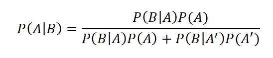 (1)
(1) An equivalent simpler form is using joint probabilities, or intersections:
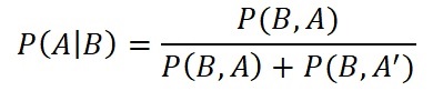 (2)
(2)
Version 2 is useful to understand bayes rule using the Venn diagram as explained further below. The simple version is:
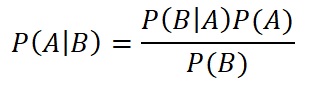 (3)
(3)
In formula 1 on the left is a conditional conditional probability, such as P(A|B) meaning "the probability that event A occurs, given cause B". The P(A) is here the prior probability, or P' (P prime). This can be subjectively estimated, with or without counts of previous cases. The event B stands for the "new information". B-prime (B') means "not B", also written as ¬B. We use the ' sign (prime) for "NOT" for simplicity. If we do not know whether B has occurred or not, all we have is the prior probability. If event B happens, the probability of having condition A changes into a posterior probability, P" (or P double prime), which is P(A|B).
The bayesian approach led to a heated discussion amongst statisticians, partly because of the element of subjectivism in estimating prior probabilities. For some "probability" is only the ratio of two counts, or the frequency of an event divided by the total number of events. The subjective probability is then nothing more than a "degree of belief". For an interesting account of the history of rejection by the "frequentists" and acceptance of the bayesian method by the "bayesians" I recommend the book by McGrayne (2011).
The Bayesian application seeks to optimally combine information from two sources:
- "Prior" notions of what is likely to occur in general, and,
- "New information" that will change our prior notions, according to probabilistic rules.
The result is denoted as "posterior" and this forms the "update" of the prior information.
The prior information can be completely subjective, but it is better to have some database to tabulate and count experience. Then we can better specify prior probabilities or distributions.
Many decisions taken in daily life use a non-formal bayesian logic: If you go for a walk, you either take an umbrella, or you dont. When you open the curtain and see a dark cloudy sky, you adjust your prior probability about rain, which is some meteorological experience to a posterior probability that is higher than the prior.
Exploration is typically a process where we slowly gather information. In a virgin area, it will be difficult to know if source rocks are present. Now we could, in despair, say that we have no idea at all about source rocks in sedimentary basins (the completely blind man in the above quote), or we could use our world-wide experience that tells us that basins are more likely to contain at least one source rock than not ("half-blind", because this data is very general and may not really be representative for our particular virgin basin).
New information may come in the form of geological age of this virgin area, say Jurassic to Cretaceous. Undoubtedly, this will affect our prior in a positive way.
It is this process of adjusting our views and probabilities at every step when new information becomes available. In the process a prior becomes a posterior, which in the next phase of updating becomes a new prior, and so forth.
Graphical explanation with a Venn diagram
A graphical explanation of Bayes theorem is a Venn diagram. We take an example from the Dutch North Sea. Gas can occur in both the Permian Rotliegend as well as in the Triassic Buntsandstein. The source is the deeper Carboniferous. The observed success rate in the Bundsandstein is overall 20%. we take this as a prior probability of finding gas in the Bundsandstein (Bunter). Permian salt separating the Permian from the Triassic is not everywhere present, either non-deposited, or removed by halokinesis. This allows migration from the Carboniferous source to the Bunter, but a proper salt seal is likely to prevent this migration.
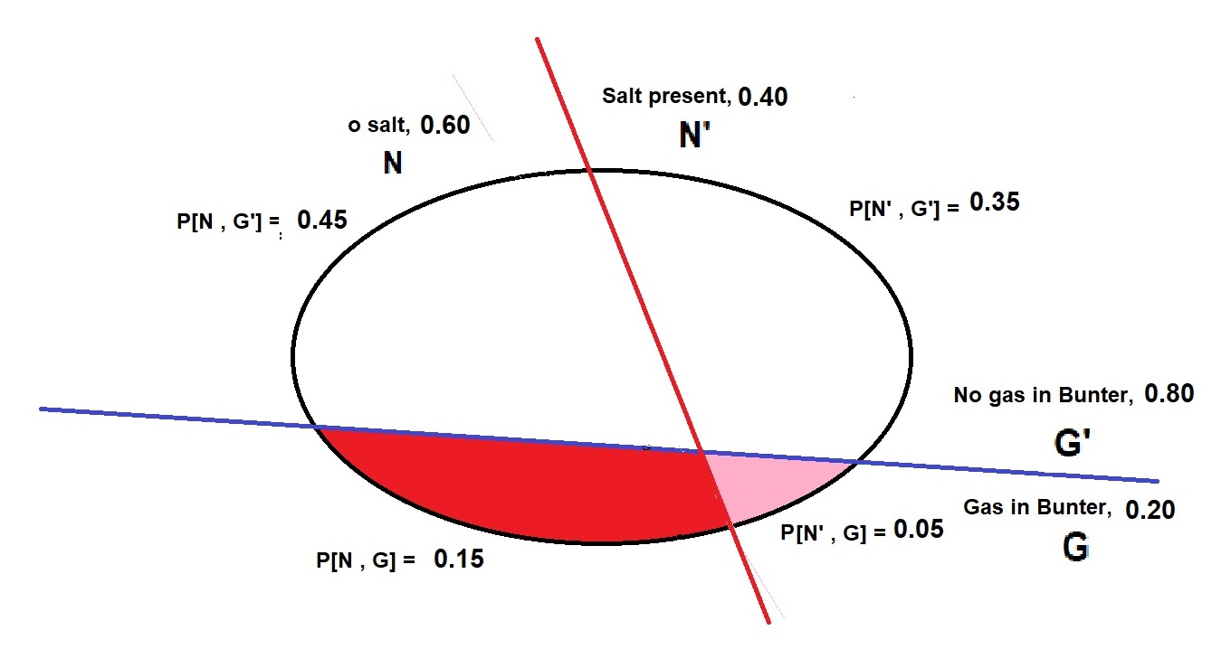
The total area of the diagram is equal to one. The four areas divided by the red line between N (salt) and N' (no salt) as well as the blue line separating G (gas in Bunter) and G' (no gas in Bunter), represent the joint probabilities. How did we estimate these areas? By counting the experience from the drilled prospects. What we are interested in is the posterior (conditional) distribution P"= P[G|N]. Having the joint probabilities as areas in the diagram, we use bayes-formula 2 (intersections) to get the conditional probability P[G|N]. We also show the calculation in numbers.
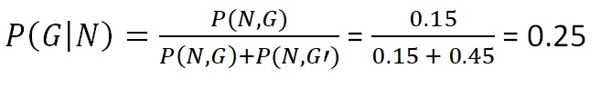
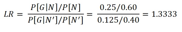
We can also rewrite formula 1 with our letters and numbers;

Note that P[N] represents the whole N area or 0.60. It is also the denominator in formula 1, as it is the sum of the two areas in N, white (N) and red (N).
Here we see that P[N,G]= 0.15 can be expressed as the area P[N] times the fraction that the gas area occupies in the N part of the diagram, so only looking at the area left of the red line, or with P[N,G] calculated using the areas in the diagram below the blue line. Finally we rewrite the simple rule as follows'
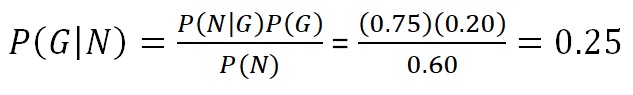
So the prior P'[G] of 20% is upgraded to P[G|N] or P" = 25% by the no-salt "new information", here called N. In the alternative situation, with salt (N'), the probability to find gas is downgraded to 12.5%.
What if the conditions G and N were independent? The joint probability areas would be different, the red and pink areas would have a ratio equal to the ratio of the N and N' areas, with the effect that the posterior probability would be equal to the prior.
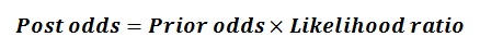
In Bayes parlance we want a "posterior probability" P" from the combination of the "prior probability" P' and the new information in the form of "likelihood ratio" P, by some called "bayes factor". The easy way is to use "odds" (a typical bookmakers' term) as in the formula in words above, where the odds associated with a probability P is P divided by (1 - P). This ratio is normally the ratio of two probability densities, see for instance the bayesian discriminant analysis. The Bayes rule can be written in words as follows:
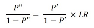
The odds-formula for the above example is:
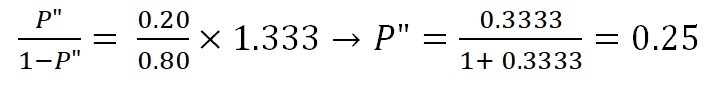
In the case of independence of N and G, the likelihood ratio would be equal to one and P"= P'.
Newendorp (1971) suggested the use of the bayesian method. In the appraisal systems that I developed for prospects and basins/plays, I used bayesian logic as far as practical. The applications are the following:
Updating various prior probabilities by a local count of cases. These involve, for instance, the probability of having HC charge for a trap ("P[HC]"), The conditional probability of having oil, given there is HC charge ("P[O|HC]"), etc. Based on bayesian discriminant analysis and Beta distributions. See also the description of the Gaeapas Full Material Balance model.
As we have only point estimates of POS for the prospect, the probability density function of POS is formed by two spikes at 0 and at 1 and a likelihood ratio as the ratio of the height of these spikes.
Updating a distribution of a variable. Uses the normal and lognormal prior and posterior distributions. Can be applied to many of the quantitative variables in prospect appraisal. When evaluating prospects in an play, a fair amount of exploration drilling may have taken place. From the results it is possible to obtain an average success rate (sometimes called "base rate"). In case this seems not to be constant in time, a creaming analysis has to be made, giving a best estimates for the near future of this average POS value. (Note that this POS is not the so-called "Play risk". The latter is the chance that "at least on discovery will be made in the play".) We take the play average success rate as the prior. This means that if we had no geological information about the prospect, such as charge, trap, seal, etc. then we would assume the prior as the POS of the prospect.
If we may consider that the geological parameters of a prospect are assessed quite independently from the total play knowledge, the total POS of the prospect will usually differ from the play average POS value. It forms "New information".With a set of prospects in the play, it may occur that the mean POS of the prospects is, for instance, much higher than the play POS. Are the prospect POS's overestimated? If it is believed that this the case, a bayesian update of the prospect risk may be advised. We use the bayes update with the "odds formula".
Example:
Assume the play P'= 0.420 and the prospect POS P = 0.700 (prospect odds = 0.700/0.300), resulting in P" = 0.628, so the prospect POS is brought nearer to the play average POS. In the example given by Milkov (2017) with some 25 prospects conclusively drilled, the correspondence between the actual and predictive is much better after the above-mentioned update of POS. However, the question remains if we can assume that the geologists making their prospect POS assessment have not already in some subjective way used the Play prior information, in which case the "update" process would inadvertently cause a bias up or down.
Application in play and prospect appraisal