Hindsight Analysis
"Success has many fathers, but failure is an orphan"
Old proverb
Many examples from exploration have shown how important a detailed analysis of a disappointing wildcat can be. An interesting story is that of the Fahud field in Oman (Tschopp, 1967), where a very disappointing well turned into a giant field. But also successes may have been systematically over- or under-estimated.
Hindsight analysis (also called "dry hole analysis" or "Post Mortem" in a more negative way) is here the statistical investigation after prospects have been drilled, by comparison of results and predictions (Nederlof, 1984). Because of the probabilistic nature of the estimates before drilling, such a comparison is far from straightforward. Basically a single number, the outcome, has to be compared to the expectation curve before drilling. But more often and more meaningful, a number of prospect outcomes is compared with their corresponding expectation curves.
Why would we bother to make such comparisons? There are few good reasons:
- Giving useful feedback to the explorationists who made the assessment.
Possibility that their subjective judgment on input variables is biased. - Learning about possible flaws in the geological model that was applied.
- Adjusting forecasts of discovery.
If the outcome of a single prospect has to be compared to the expectation curve before drilling, the possibilities for testing are very limited. Obviously, if the outcome falls completely outside the range of the expectation curve, there must be something wrong. But generally the situation is less clearcut. The most simple approach is to use the cumulative distribution and pick the percentile where the actual outcome is situated. If it is far in the right tail of the distribution, say at the 5% or at less percentage, the deviation can be regarded as significant, and indicating underestimation. However, if the outcome is zero, and the expectation curve contains many zeros (POS << 100%), we cannot conclude much, although overestimation may be indicated. Considerably more can be learned if a number of expectation curves can be compared with the corresponding drilling results. The analysis will be fourfold:
(1) Probability of success
(2) The volume in the case of success
(3) The total sum of volumes discovered and the sum of expectations
(4) The ranking ability.
Probability of success
With a small number of drilled prospects, a precise calculation of the distribution of successes is available, if the prospects can be regarded as independent (Nederlof, 1994). The mathematics are more complicated than in the case that all the individual POS values are equal. In the latter simple case, the binomial distribution, as is, is sufficient. If r is the number of successes out of 5 prospects, the probability to have r = 5 successes is:
and more complicated for the intermediate values of r. A program in the Gaeatools set does these calculations of the frequencies and provides the cumulative distribution (cdf) of r. For higher numbers of prospects an approximation is used. This is based on the normal distribution with a mean and variance as follows:
Once we have the cdf we compare the actual number of successes with this "expectation curve" of r. If the number of successes is significantly less than the expected number, the appraisers were too optimistic, and a significantly higher observed success rate than suggested by chance, the appraiser were too pessimistic. Consider the following case with 8 prospects. The individual probabilities before drilling were:
| 0.23 | 0.35 | 0.12 | 0.38 | 0.03 | 0.57 | 0.14 | 0.41 |
With this data the distribution is as follows, with emphasis on the case of r = 5 .
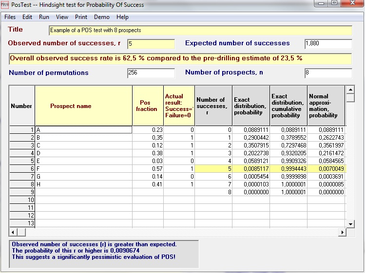
The difference between the normal approximation and the exact distribution is minimal, despite the still small number of prospects. This is graphically shown below in the cdf and the histogram (pmf):
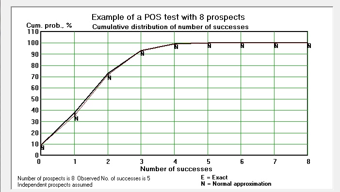
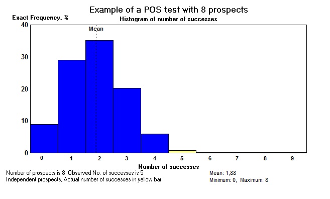
We see that the expectation of the number of successes is 1.88. So, 5 successes is significantle more than predicted. With POS values, as usually fairly low, it is easier to obtain significant pessimism, because of the thin right tail of the distribution. To prove people were overoptimistic is more difficult. If all 8 prospects were dry, we would not have a significant result (p = 8.9%).
and graphically:
I once checked the outcome of 20 ventures that had been estimated by various prospect appraisal methods. I had the expectations and the actual results. The sum of the actuals was about seven times smaller than the sum of the expectations. A rather typical sign of over-optimism. Now the evaluations in this example were far from thorough, and date from a time that not too much attention was paid to get it right. A later example, based on more sophisticated appraisal is from Oman.
The procedure is:
The total sum of volumes discovered and the sum of expectations
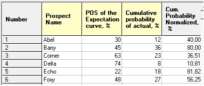
At this stage we can compare a single number (the total actual) with the expectation curve (MC summation). The result for the 16 prospects evaluated and drilled in Oman were:
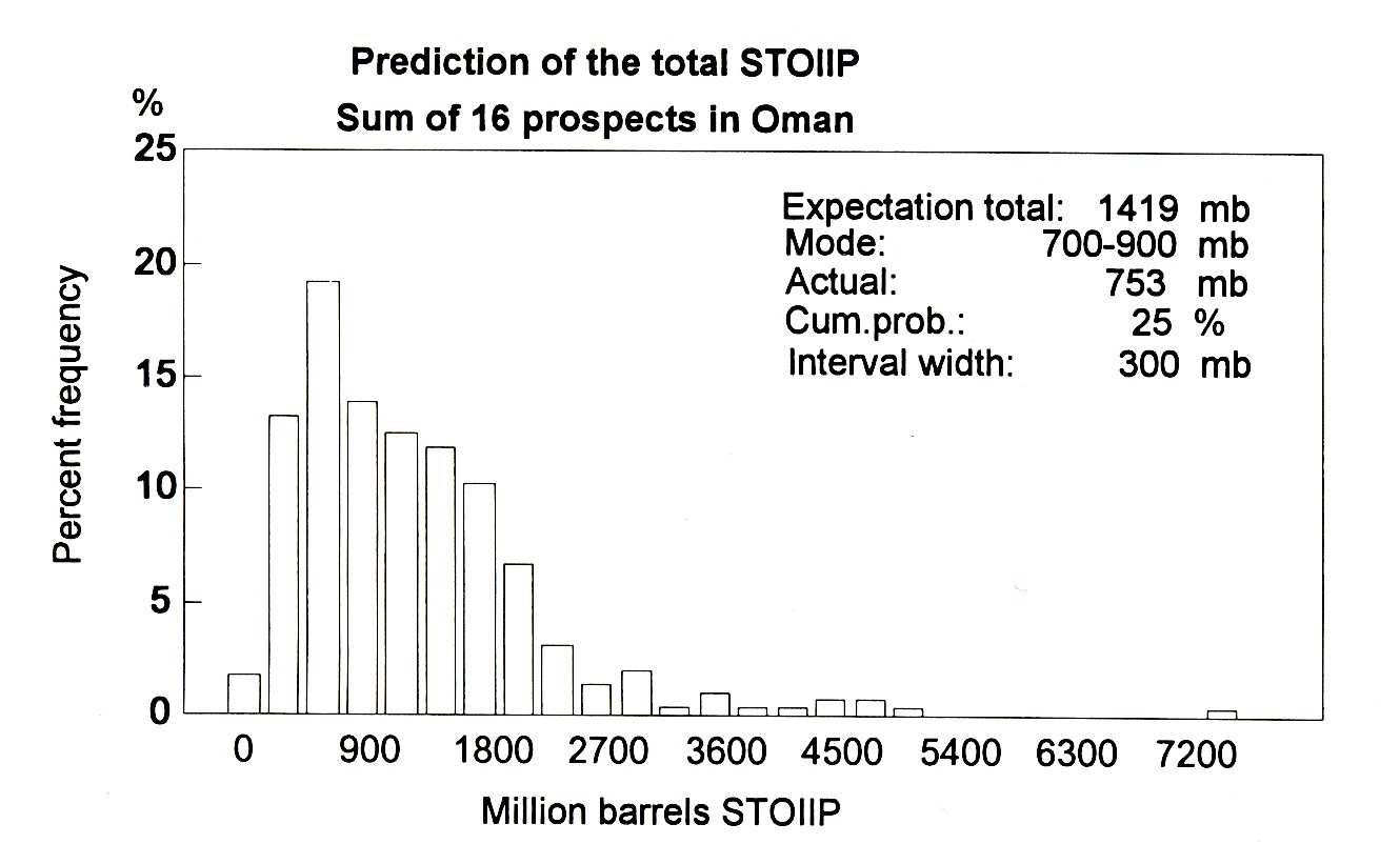
Note that on purpose the MC addition was done with independence. If some dependence had been included, the test would have more difficulty to detect bias in the appraisals, then being less sensitive. The result shown in the figure puts the actual at the P25 in the expectation curve. As it happens, also in the modal range. Therefore no indication of bias, despite the mean expectation being almost twice the actual. The exercise also shows that adding 16 skewed expectation curves does not yet generate a sum distribution that is normal.
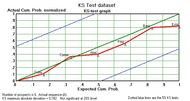
Ranking ability
Even if the Pos, the KS and the Sum test have found everything in order, we still do not know whether the appraisal system can rank prospects in an optimal sequence. This property is "ranking ability" and is quite independent from the other tests. The test devised for this purpose is the
Most CAT curves will befound between the two extremes: the best possible (only practically possible if you have a sixths sense) and the worst possible (suggested by the Devil, and detrimental to the Present Value of the discoveries). In order to test a sequence of prospects we need a test statistic that measures the deviation from the "random drilling" line. This is:
We can also calculate the cumulative area under the observed curve and divide this by the total cumulative discovery. This we denote as the CAT-r, a kind of correlation coefficient, that can vary from -1 to +1. It would be zero for the (average) random drilling line. For the significance test, however, we use the above CAT statistic. It can be proven that this statistic has a mean of zero and a variance of
Where x is the set of n actual values. The variance of the x's is calculated considering that the n values form a population in the randomization. The total number of permutations being n!. Even for small n the sampling distribution of the n! possible CAT values tends to normality. The figure below shows a case where only 9 prospects with expectations ranging from 0 to 50 mb are permuted 20 times. The resulting distribution of that sample follows rather nicely the normal.
A real case was published by Sluyk & Parker (1986). In a period of 10 years 165 prospects had been appraised by the Shell prospect system (Sluyk & Nederlof, 1984) and also had been conclusively drilled. The result of the CAT test was:
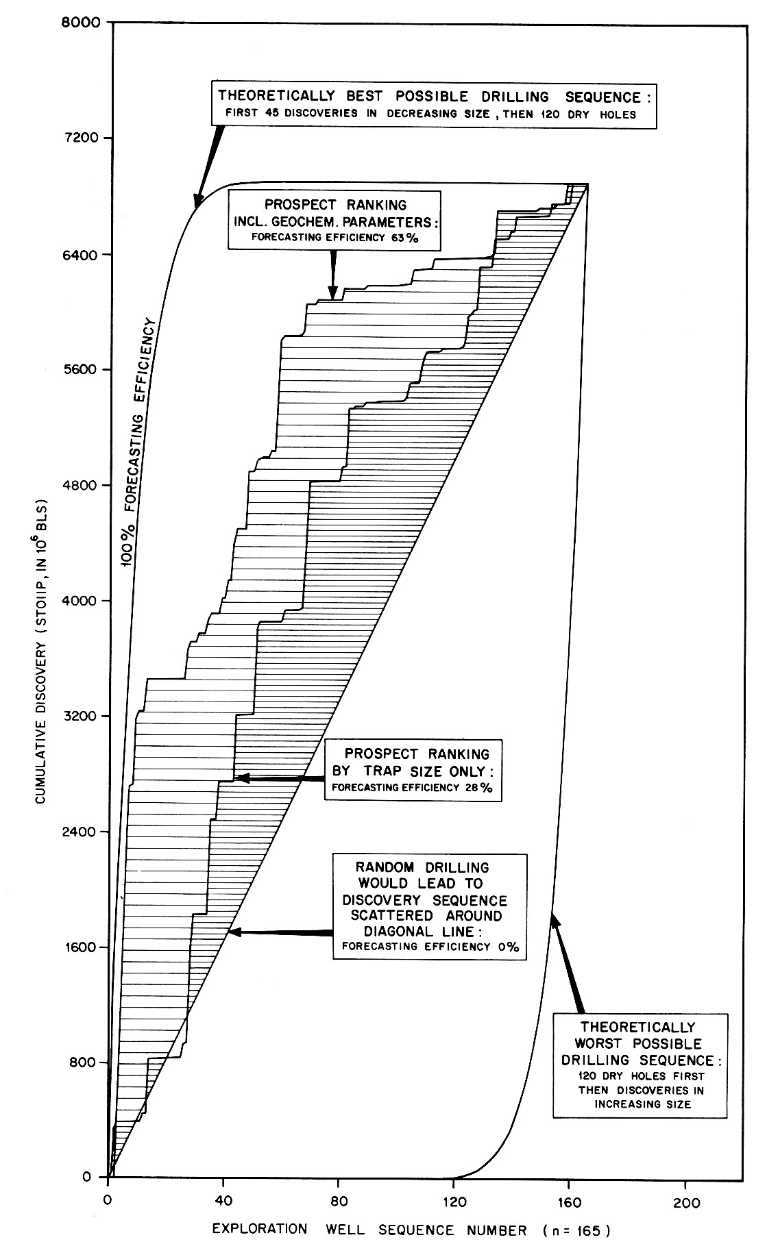
For smaller sample sizes, the CAT test for ranking ability is supposedly better than a simple rank correlation (Spearman or Kendall) because CAT uses more information and does not require a correction for tied observations. Tied observations are in this case due to a number of zero outcomes, the dry holes. For the above large sample the significance level is about the same.
An interesting aspect is the indication of the usefulness of including the geochemical/geological data, above the practically pure structural information (at the time of the above analysis) from seismic methods.
It is not easy to find enough reliable data for hindsight analysis, but the learning value of such an effort is high. Here is a rare example from a publication by Milkov,(2017): The 25 data were analyzed with much care, as definitions of what is an exploration well may be inconsistent sometimes. The result is shown below:
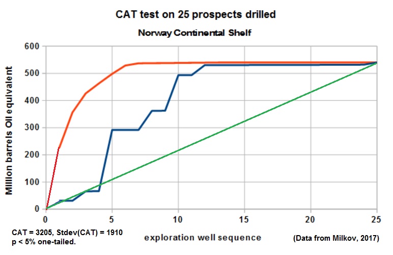
When we apply the CAT signoificance test to this data set, the CAT statistic = 3204, the standard deviation = 1910, which gives, using the t-distribution with 24 d.f., a one-tailed probability of 0.0476, just significant at the 5% level.
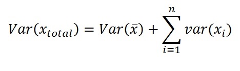
What to do if the outcomes are so recent that we only have a probabilistic estimate of the volumes in the discoveries? We may safely assume that the zero outcomes have a variance equal to zero. However, the non-zero volumes are uncertain and we have to account for this in the variance of outcomes. The variance of x in the formula for the CAT variance is adjusted according to the following formula, which states that the variance of x in the case of uncertain x-values is the variance of the mean x values plus the sum of the individual x variances:
In the above example from Norway we do not have estimates of uncertainty. However, it is easy to see that, even with a moderate uncertainty about the outcome sizes, the variance of x will be larger and the above significance level not reached.
Top