Lognormal Distribution
- The distribution
- Generation process
- Parameters
- Natural of Briggs logarithms?
- Threepoint estimate of a lognormal
- Swanson's rule
The lognormal distribution is found to the basic type of distribution of many geological variables. When the logarithms of values form a normal distribution, the original (antilog) values are lognormally distributed. It is a skew distribution with many small values and fewer large values. Therefore the mean is usually greater than the mode. In geology, many processes lead to a lognormal, so often that it has been said the lognormal is the normal of geology. The lognormal is important for prospect appraisal because a variety of the geological factors are so distributed. Also in petrophysics, the lognormal is well-known for pemeability and the semi-logarithmic permeability/porosity plots. In sedimentology in grainsize distribution and bed-thickness distributions. Source rock samples along a borehole usually give a lognormal distribution for the TOC values.
The generation process
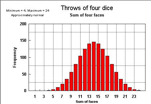
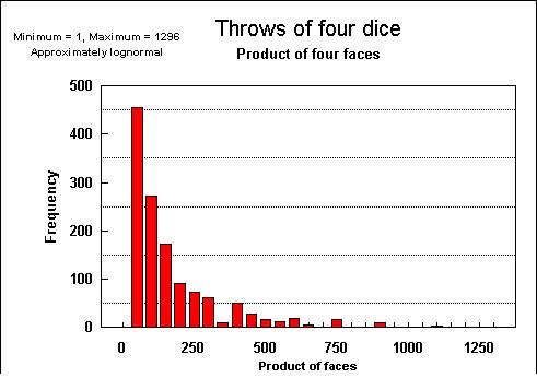
Multiplication of numbers can be done by addition of the logatrithms and taking the antilog of that sum. This principle helps to understand the nature of the lognormal distribution. We consider first a process that does not involve multiplication, but addition. We throw four dice and each time we record the sum of the faces. The numbers can vary from 4 to 24. The distribution of these sums of faces tends toward a normal distribution, (although it is a discrete distribution):
| Sum >>> Normal | Product >>> Lognormal |
|---|---|
 |
 |
The generative process leading to a lognormal distribution was explained by Gibrat (1930) and called "the law of proportional effect". It is also closely related to the power law distribution (Zipf, Pareto) and this is explained in a readable paper by Mitzenmacher (2003).
The proportional effect could possibly operate in biology, in the description of growth of organisms. If the amount of growth is proportional to the size of the organism a lognormal distibution of sizes would be generated. If field reserves are reported, but not expectations of ultimate recovery, fields would grow like organisms, by appraisal wells and subsequent updates of the reserve numbers.
However, field Ultimate Recoveries, "field sizes", are roughly the product of a set of variables, such as length, width, height of a trap, porosity, reservoir thickness, hydrocarbon saturation and recovery factor. Even if these variables would have a symmetrical distribution, it would not be surprising to see a lognormal distribution for the product, just as we saw in the experiment with four dice.
A different explanation for a lognormal distribution is a breakage model. The most simple one-dimensional model is a series of events that occur at random in time. So, for a given time interval the events are distributed as a rectangular distribution of moments. Then the intervals between event tend to be distributed as an exponential distribution. This situation is known from telephone research for incoming calls on a very small time scale, but on presumably a much larger time scale for the arrival of turbidity currents.
In three dimensions, if a material object like a stone is crushed, the size of the pieces are skewly distributed. Crushing a rock, the breakage can be simulated by breaking a given length into smaller pieces at random. This would give an exponential distribution of the parts, as in the time sequence. If the parts themselves are broken in turn, a different size distribution results, and possibly the lognormal. A very large number of papers have been written on breakage models and the size distributions that result (Epstein, 1945).
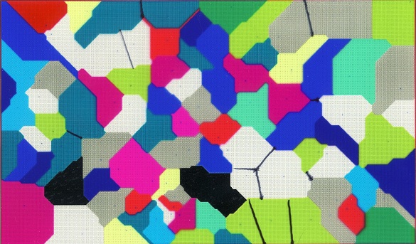
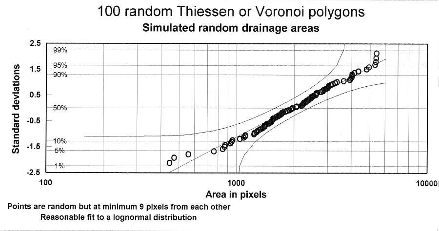
In the petroleum system similar processes are at work in two dimensions: a tectonic style subdivides an area in parts which contain traps. Each trap has a drainage area, and these form roughly a breaking pattern. Because there is some non-randomness in tectonics, a size distribution of drainage areas results that is not a J-shaped exponential distribution, but more like a lognormal. As such a distribution could work through into the hydrocarbon charge to traps, a lognormal can be expected for underfilled traps. A similar process may involve the trap sizes themselves, especially if faults dissect the area into parts. This process can be modeled with random polygons. In this case we assume that a set of randomly located points in area are nuclei for the polygons. The boundaries between adjacent polygons are than at the middle distance to the starting point. Here is an example as a coloured map and next the lognormal dsitribution plot of the coloured areas:
The parameters
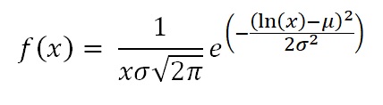
The probability density (pdf) is:
Cumulative Distribution Function>
The Cumulative Distribution Function (cdf) can be calculated analytically, like the normal distribution.
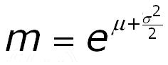
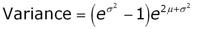
| Mean | Variance |
|---|---|
 |
 |
 |
 |
In exploration prospect appraisal, the usual statistical procedures to arrive at an estimate of the "unrisked" volume of hydrocarbons that might be found, leads to a skew distribution, as explained above by the set of variables that are multiplied together. In further analysis, involving several prospects and economic cutoffs, the shape of the distribution of such volumes is important. Assuming a normal distribution is certainly wrong. Often a lognormal distribution is assumed. In practice it is found that in addition of prospect estimates, the normal will underestimate, while the lognormal will overestimate. It seems that a triangular distribution may give more reliable results.
The cumulative lognormal distribution can be conveniently shown on log/probability paper, which is often done when studying fieldsize distributions for basins, see Fieldsize distribution theories.
Using logarithms to base 10 rather than e.
As it is somewhat inconvenient to work with the natural logarithms to the base e= 2.718.., it is useful to know the consequences of switching to the Brigg's logarithmes to the base of 10, or 10Log's.
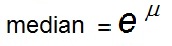
Above we have given the mean of the lognormal as
We can rewrite the above as:
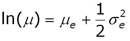
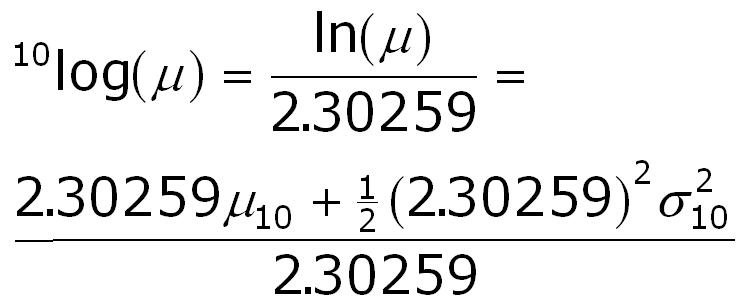
The subscript "e" indicates that the parameter was calculated with the natural logs, while the subscript "10" is for the 10Log data. The relationship between the means of natural logs and Brigg's logs is:
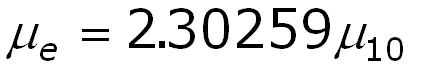
because:
Also:
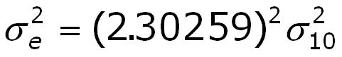
and the relationship for the variance is:
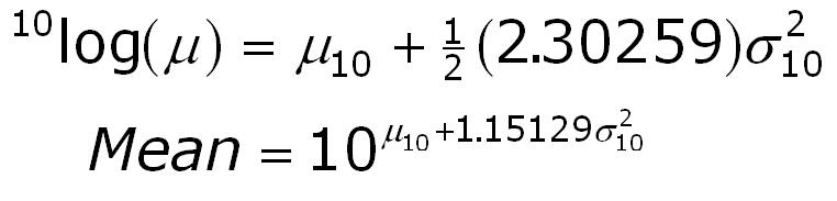
Finally we arrive at:
A three-point estimate of a lognormal distribution
For a prospect appraisal program it may be required to give the parameters of a lognormal distribution, i.e. the mean and standard deviation in terms of natural or Brigg's logs.
The mean and standard deviation in 10Log terms may be difficult to estimate. Therefore an alternative input is similar to the triangular distribution input: Low, Mode ("most likely") and High. The example below shows the (Gaeapas) input in linear numbers on the right and the resulting lognormal logarithmic parameters on the left. The relationships between the triangular and lognormal distributions to calculate the mean and variance required for the simulation are found (making gratefully use of the formulas for the lognormal mode and mean which give two equations with μ and σ2) as:
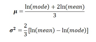
mode is the mode of the triangular and mean is the mean of the triangular. ln stands for "natural logarithm".
To have a successful estimate of the two lognormal distribution parameters to the three triangular parameters, it is necessary that
If not, the skewness of the LN would be positive instead of the negative skewness required. (The variance would become negative, which is impossible).
| Low | Mode | High | Mean | Variance | St. deviation | |
| Triangular | 5 | 12 | 23 | 13.3333 | 13.1667 | 3.6286 |
| Lognormal | 5.9455 | 11.9987 | 27.0551 | 2.5555 | 0.0702 | 0.2649 |
In the second row of the table above, the first three parameters are the result of 1000 MC cycles, showing the approximation to the triangular input. The parameter further to the right are the parameters of the lognormal distribution.
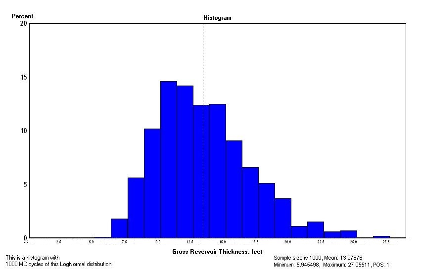
Note that the lognormal fit to the Low, Middle and High honours the mode of 12 but extends the distribution to the right to a range to 27. The theoretical range for the lognormal is 0 to +infinite. The MC sampling attempts to produce that range, but obviously cannot do so fully.
In the case of a percentage input (e.g. porosity) it would be awkward, to say the least, if the extended range produces negative values. In such case the tail ends of the distribution below zero (not possible for the lognormal) and above 100% should be distributed over the 0 to 100% range proportional to the frequencies of the values in the 0 - 100% range.
Many skewed data distributions in nature follow a log-normal distribution. The pdf of the log-normal is more complicated than that of the normal distribution, but if we consider the parameters derived from the logarithms of the observations, such as the mean and the variance we are back to the formula for the normal distribution. We should note, however, that the mean of the logs of values xi translated to linear numbers is not the same as the mean of the xi! This is a problem that may be encountered in the interpretation of permeability/ porosity plots on semi-logarithmic paper. The scatter of points on such a plot may suggest a curve or line relating permeability (k) to porosity. In order to predict the permeability at a given porosity, we cannot just read off the permeability on the Y-axis, but we have to take the scatter of k-values around the curve into account (see the above formulas).
It is applicable to a lognormal distribution, if the variance is not too great. Now the question is "what is too great?". A simple rule is to calculate the ratio
For a true lognormal distribution, Swanson will give a too low mean. The difference is small if the above ratio remains under 2.5. The following graph illustrates the % error for a true lognormal. In practice the errors are less for more symmetrical distributions, somewhere between a lognormal and a normal.