Normal Distribution
The normal distribution is the most common type of probability distribution, found in many widely different branches of science. It is usually ascribed to Abraham de Moivre (1667 - 1754), but very often referred to as the Gauss distribution. De Moivre was assisted by James Stirling (1692-1770) who calculated the constant which is required to make the area under the density curve equal to one:  in the formula for the density distribution (pdf):

The "standard normal distribution" has a mean of 0 and a variance of 1.
Unfortunately, the Cumulative Distribution Function (cdf) has no analytical expression and the cumulative probabilities have to be approximated numerically. The same holds, of course, for the inverse normal distribution. To generate random normal numbers from random uniform numbers several algorithms have been invented. Thomas et al. (2007) give a very good overview.
A simple one I used, when no great accuracy is required is the following: Take twelve uniform random numbers, add them up and substract 6 from the result. Why? Because a uniform random number has a mean of 0.5 and a variance of 1/12. Summing the 12 independent numbers, the result is a mean of 12 times 0.5 is 6. The variance is the sum of variances: 12 times 1/12 is one. So the result minus six gives a standard random normal variate with mean zero and variance one. The disadvantage is that the tail ends of the distribution are not very well modeled in this way.
One of the most elegant ideas has been suggested by Box & Muller, 1958. The algorithm uses two independent random numbers between 0 and 1 to generate two gaussian independent numbers at a time. A single nomal distribution is one-dimensional. If we multiply two such distributions, we obtain a two-dimensional distribution. Take the simplest expression of a normal density and multiply two of these:
The exponent R2 = x2 + y2 is representing a circle:
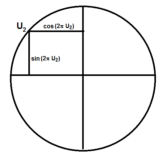
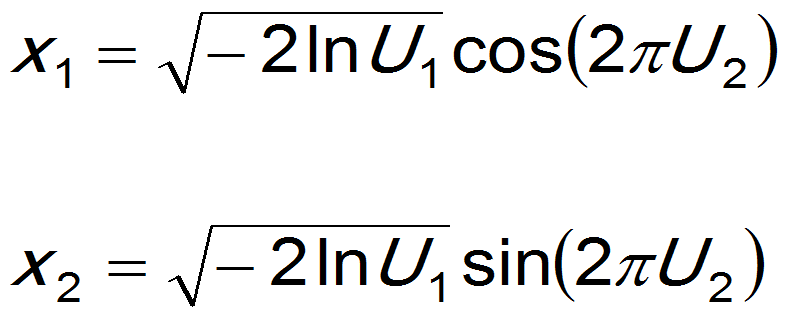
Using the two dimensional coordinates, and using another independent uniform variate U1, the following formulas give two independent normal random draws from a standard normal distribution, i.e. with mean = 0 and variance = 1. The pairs of normal random numbers are the coordinates of points in a bi-variate standard normal distribution:
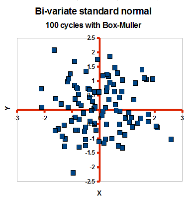
In the above cloud of points we see no correlation, otherwise the cloud would be elliptic in shape: the random draws in a pair are independent. Here is a sample generated by the algorithm:
For an explanation in more detail and the optimization of the algorithm for computing see Wikipedia for "Box-Muller transform".
The normal distribution is not so common for geological variables, although porosity uncertainty can usually be described by it. It has been said that the lognormal is the most "normal" distribution in geology. Examples of the data that do not fit the normal distribution are: Total Organic Carbon %, grainsize, drainage area size, fieldsizes, etc..