Probability
The notion of probability was possibly first developed by
Gerolamo Cardano (1501-1576), an Italian Renaissance mathematician, physician, astrologer and gambler. Cardano was notoriously short of money and kept himself solvent by being an accomplished gambler and chess player. His book about games of chance, Liber de ludo aleae ("Book on Games of Chance") , written in 1526, contains the first systematic treatment of probability, as well as a section on effective cheating methods. It could be that he was inspired by a 12th Century poem containing calculations about a game with dice.
(from Wikipedia).
Contents
- Frequentistic probabilities
- Subjective Probabilities
- Risk
- Combining Probabilities
- Conditional probabilities
- Prior and Posterior Probabilities
- Influence of information on a probability estimate
The importance of probability estimates is mainly the "Probability Of Success" (POS) as used in prospect appraisal.
Frequentistic probabilities
Assume we cast a die. The possible outcomes are 1, 2, 3, 4, 5 or 6. We repeat the experiment and count the number of cases that 6 comes on top. That is the frequency. An experiment with 60 throws of the die will, theoretically give ten times a 6. The frequentistic probability is then 10/60 = ~ 0.167. This concept of probability depends on repeated experiments. In the practice of geology, uncertainty may exist about the "state" of a situation, which is known by God, but not by the geologist. If he does not have a database with known similar situations, he does not have any frequencies to use. But he does have a subjective feeling that th�s state is more probable than th�t state in this situation. Therefore we will accept the concept of a subjective probability, even in a basically quantitative appraisal model.

| Degree of Confidence | Weight factor |
|---|---|
| Impossible | 0 |
| Extremely unlikely | 1 |
| Very unlikely | 2 |
| Unlikely | 4 |
| Likely | 8 |
| Very likely | 16 |
| Extremely likely | 32 |
| Certain | Infinite |
An experiments with 30 subjects allowed to estimate the relative likelihoods of successive steps in this scale of degrees of confidence". Interestingly, subjects would switch to the next higher term, or the next lower, when the (true) likelihood changed with a factor 2. This result is consistent with biological research on stimuli, where, for instance, increased pressure on the skin will trigger a response only when the pressure is doubled, and therefore appears to justify the above weights.
The mechanics of using this scheme is to calculate the expectation from the scores assigned to the 8 classes, using these weights. In the case of a probability we would end up with a single estimate of the probability, but one which should better represent a subject's thinking than asking immediately for this single number. Note that the mechanism should return zero if there is any score assigned to Impossible, or 1, if any score for Certain. These extremes would simply override any intermediate statements. Although the method might appeal to some because of the use of common words as a starting point, it is not proven that it has any advantage over using a simpler approach.
In practice, the above scheme does not deviate significantly from one in which we let a geologist start from a numeric scheme of estimating a histogram. First the histogram classes are fixed. For a probability one could use e.g. 10 classes of width 0.1. The the user should assign scores subjectively to these classes. Their scores would be the weights to be assigned to the class-midpoint. Here the scores are percentages, the sum of which should be 100.
This method is the "user-defined histogram" or "UDF". The class boundaries are always chosen to be relevant to the variable to be estimated.
Here is an example:
| Classes | 0.0 - 0.1 | 0.1 - 0.2 | 0.2 - 0.3 | 0.3 - 0.4 | 0.4 - 0.5 | 0.5 - 0.6 | 0.6 - 0.7 | 0.7 - 0.8 | 0.8 - 0.9 | 0.9 - 1.0 |
| Scores | 0 | 5 | 15 | 50 | 20 | 10 | 0 | 0 | 0 | 0 |
This statement would give a probability of 0.365 by calculating the weighted mean value of this histogram (expectation)
([5*0.15 + 15*0.25 + 50*0.35 + 20*.45 + 10*.55] / 100 = 0.365).
There are some drawbacks to this approach. In the example it is impossible to get any probability less than 0.05, or greater than 0.95. This is quite unrealistic. However, how good are we to estimate extreme chances? My experiments with a a fairly large number of subjects showed that, when asked to give confidence intervals of some variable to be estimated, these were most of the time too narrow. That is: too many true values fell outside their 95% confidence interval (it should be only 5%). Even worse are results for the 99% confidence interval. This is somewhat in contrast with the extremes of the probability range in the figure given above: People are giving a much narrower range for probabilities at the extreme ends, which means there is consensus about what a particular word means. However, consensus does not mean we are right!
For estimating a value, such as an average porosity, the UDF appears straightforward. But what about estimating a probability as we did in the above example? Does it make sense to be uncertain about a probability? To answer that question we have to return a moment to the frequentistic probability. If the probability is calculated as the ratio of a number of particular events over all events in a limited sample, we can use statistical rules to establish how uncertain our probability estimate is. In the geological practice, we rarely have such data to lean on. Some statisticians would say that we have no "probability" at all if we estimate it subjectively (or if you wish intuitively), based on some experience database in your brain. They would call it "degree of confidence" a term that we already used above for the scores. In practice, such distinction is not too important. This leaves us with the fact, like it or not, that there is usually uncertainty about an estimated probability (P) or about a degree of confidence.
In further use of these probabilities it may matter whether we use a single number for P or a distribution ("histogram") of possible P values.
Capen (1976) wrote:
'Having no good quantitative idea of uncertainty, there is an almost universal tendency for people to understate it. Thus, they overestimate the precision of their own knowledge and contribute to decisions that later become subject to unwelcome surprises'.
In this paper he presents an experiment with general questions and with estimating the number of beans in a jar (951). The result shows that, if subjects are supposed to bracket the true value with a 95% confidence range, quite often the whole subjective confidence interval does not cover the true value, for instance "400 to 500". My own experience during courses showed similar results.
My definition of the word "risk" is probability of failure. Hence it is the complement of the probability of success ( Risk = 1 - POS). Risk is the upper part on the vertical axis of the expectation curve, down to where the curve turns off to the right.
In prospect appraisal risk is used in the sense of "straight risk", the probability that a certain essential ingredient of the petroleum system is absent. For instance the risk that there is no viable reservoir. The straight risk is usually a subjective point estimate of a probability. The term "risk" is sometimes used for "uncertainty", probably not a good idea. The term risk is important in the definition of the MSV, because the is the mean of the "unrisked" set of possible outcomes, or unrisked mean.
Combining Probabilities
In some cases probabilities are added. For instance: How many times do we throw more than 3 with a die? That is P(4) + P(5) + P(6) = 3/6 = 0.50. Note that we assume the die to be honest and the events of throwing a die are independent events.
In prospect appraisal the more common situation is that we multiply probabilities. When a number of conditions affect prospectivity, the product of the individual probabilities gives the final probability of success. This simple solution requires that the individual factors are independent. If not, the covariance of amongst the factors have to be taken into account and this may not be practically possible. A mistake I have come across is that the mean of the individual probabilities (average) is used instead of the product!
These probability rules are important when evaluating a concession with more than one prospect (Damsleth, 1993), to arrive at an expectation curve for the concession. This involves the addition, or "aggregation" of resource estimates.
In combining probabilities it may matter whether we use a single number for P or a distribution ("histogram") of possible P values. Here is an experiment based on Monte Carlo modeling with 100,000 cycles.
Here is an experiment based on Monte Carlo modeling.
In a certain prospect appraisal scheme we use four chances of fulfillment:
- P1, Chance of having Hydrocarbon generation/migration
- P2, Chance of having a trap
- P3, Chance of having a reservoir
- P4, Chance of having retention
Probability of Success ("POS") = P1 x P2 x P3 x P4. (we call this "pf" for probability of fulfillment)
If the pf is calculated as the mean of the Monte Carlo-generated pf's, we call it "pfp".
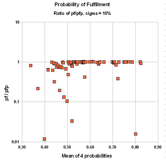
Point estimates are given for these chances. If the average of these chances is low, say 0.10, then the error made in case these chances are not exact can be significant. For instance, with a 10% uncertainty (standard deviation of a normal distribution) around the subjective point estimate, the final product of probabilities is some 25% too low!
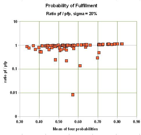
If the average chance factor is 0.8, the bias is as much as 5% overestimate for a st. dev. of 10%, 9% overestimate for a st. dev. of 20% and 26% upward bias for a 30% st.dev.
Here is the result for two cases of uncertainty in the estimates of the individual probabilities: One for a standard deviation of 10%, the other of 20%. We graph the ratio of pf over pfp versus the average of the four input probabilities:
 |
 |
In summary, the final chance of fulfillment is the product of the individual chance factors for the "ingredients" of the petroleum system. If, on average these chance factors are low, the probability of success will be underestimated, compared to a system that takes the uncertainty into account. For chance factors that average above 50%, the bias will be to inflate, or overestimate the probability of success. The correct product of the individual probabilities must be the Monte Carlo-generated pfp, because it can not be argued that our estimates of the p's are absolutely sure. Just think of a delphi exercise in estimating the four p's. There would be a lot of disagreement, finally hidden by consensus numbers. Fortunately the discrepancies are not at all extreme. Only when considering a prospect with a small probability, but a high reward, could this bias play a role.
Possibly such bias can be removed, or reduced by using a so-called "fuzzy" system (Roisenberg, et al., 2008). Then the uncertainty of the probability estimate is taken into account, but I have not seen experimental evidence that this works.
In summary, the final chance of fulfillment is the product of the individual chance factors for the "ingredients" of the petroleum system. If, on average these chance factors are low, the probability of success will be underestimated, compared to a system that takes the uncertainty into account. For chance factors that average above 50%, the bias will be to inflate, or overestimate the probability of success.
Possibly such bias can be removed, or reduced by using a so-called "fuzzy" system (Roisenberg, et al., 2008). Then the uncertainty of the probability estimate is taken into account.
Top
Conditional Probabilities
Conditional probabilities are helpful in clarifying the logic in the more complex situations. They are the "if this than possibly that".
An example of a conditional probability is P[O|HC], the probability that there is oil charge given that there is Hydrocarbon ("HC") charge. If P[O|HC]=0 it implies that only non-associated gas has migrated to the trap. Other examples are: P[FG|HC] , the conditional probability of having free gas if hydrocarbon charge is present. and P[C|FG], the probability of having condensate if there is free gas. The latter needs some criterion to define "dry gas".
In complex situations it can be helpful to show the conditional probabilities in Venn diagrams.
These terms apply to estimates of probability in bayesian statistics. A prior probability is usually a distribution of possible probability values, because we only have a vague idea of what the probability is. In an undrilled area we do not know what the success ratio will be for wildcat drilling. However, worldwide experience tells us that it may somewhere between 0.0 and 0.5, with a mean value of 0.15. For instance, as soon as 5 wells have been drilled, two with success, three dry (a success ratio of 40%), this small sample of data allows us to update our prior success rate probability to a posterior one. If we see the prior as a rather flat distribution of possible success fraction between 0 and 0.5, the posterior will be sharper, with a peak closer to the location of the sample mean of 0.4, e.g. 0.25.
I have seen several evaluation systems which, in some way or another confuse amount of information with probability. In those cases a subjective probability is thought to be dependent on the amount of information. See Duff and Hall (1996). This is not the case. The amount of information influences our confidence in the probability estimate, not its value. In principle, only the confidence in the probability guess is dependent on the quantity and quality of information available. An illustration of this principle is discussed in the description of the Beta distribution.
If additional, or better quality information becomes available, it can be simply confirmative and hence give more confidence in the earlier estimated probability. If the new information is
different from the earlier data available in the sense of of being more favorable, or the opposite, then also a new probability estimate has to be made. We may not assume beforehand that more information will increase the probability or decrease it. Peel & Brooks(2015) have noticed that misunderstanding the effect of information on POS is apparently widespread.
Related to this problem is that, in case of ignorance a probability is 0.5, because there is no evidence for an event to occur or not. To illustrate this approach we could ask "What is the probability of having elephants on Venus". We dont know, so the probability of having elephants on Venus is 0.5. This would be ignoring all kinds of background information about elepohants and, for instance, the climate of Venus... In prospect appraisal, we always use our experience, although not necessarily based on counting events, to come to a prior probability that may deviate considerably from 0.5 .
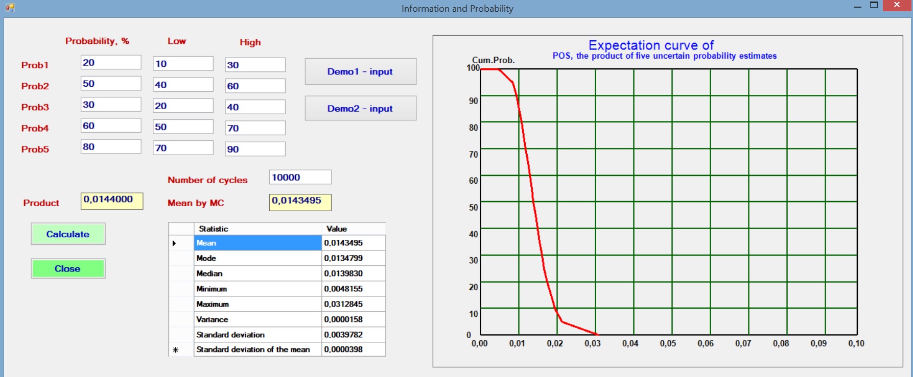
In the common case that a number of probabilities are estimated and multiplied to give an overall probability, it is interesting to see what happens if we assume a small uncertainty of the individual probabilities. To model this situation we assume that the initial probability, say Prob1 is the best estimate, or mode of a triangular distribution. The estimator also gives a Low and a High estimate to reflect his uncertainty about Prob1 and likewise for the other probabilities. Then a Monte Carlo analysis with 10,000 cycles draws from these distributions the individual probabilities and multiplies these to obtain the POS for each set of random draws of the Probs.
The results with various sets of individual probabilities shows that the resultant product (POS) is not dependent on the uncertainty (the range given by the triangular distribution). One of the trials is illustrated below.
The above reasoning does not imply that a measure of confidence/information would be meaningless. It points to situations where it might be wise to gather more information before dicision making. In that context the "value of information" plays a role.
Prior and Posterior Probabilities
Influence of information on a probability estimate