 (1)
(1)
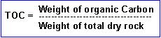
Total Organic Carbon content ("TOC") of a source rock ("SR") can be determined in the laboratory from a sample. In such analysis the non-organic Carbon content, such as in carbonates, is removed. Measuring the Carbon dioxide resulting from combustion then results after some calculation in the dry weight percent TOC.
The TOC consists of an inert part (e.g. charcoal particles, inertinite) and a part that is associated with kerogen that can be converted into oil and gas. There are various views on what the minimum amount of TOC is for qualifying as an effective SR. The author assumes that any TOC below 1.5% is doubtful to contribute to expelled oil. At low levels of TOC, oil and gas may be formed within the SR, but may not be sufficient to be expelled, a minimum amount being required for primary migration. However, the small amounts of oil generated in the SR will remain there when the SR is matured further, eventually transformed into gas that finally may be expelled. It could be argued that for gas SRs, there will be often more inert Carbon, so the threshold might have to be higher.
Because of the threshold level of TOC before effective expulsion takes place, it is important to recognize a TOC "cutoff" value based on the above reasoning, such as the 1.5% used in the GAEA50 prospect appraisal program.
Organic material that contains the TOC is lighter than the usual rock mineral components, such as quartz and carbonates. Also the speed of sound is considerably less than in the mineral grain framework. Organic material is also a poor electricity conductor, especially when it contains generated oil. These properties make it possible to detect the presence and amount of organic material in a rock from wireline measurements, under favourable circumstances. The logs that are useful in a wide variety of circumstances are the resistivity log, the density log and the sonic log.
The SRLOG program uses a combination of density/resistivity or sonic/resistivity to estimate the amount of TOC. The calibration has been made by a regression of log(TOC%)on log(depth in M), Log(Resistivity in OhmMeter), log(slowness in Microseconds/foot), or Log(Density ion Grammes/cm3). By including the depth, the resistivity is implicitly standardized to a fictitious standard temperature. This way we do not have to have access to borehole temperatures, which for the calibration data from various sourxces was not available. Sample sizes were 208 for the Sonic/resistivity method and 178 for the density/resistivity. The regressions are statistically highly significant. Nevertheless, as the application shows, a large range of uncertainty for the TOC estimate results. That is why the results show the 5% and 95% confidence limits as well as the estimates.
Density log
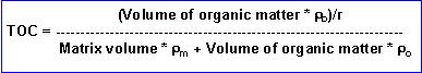
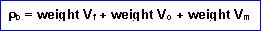
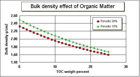
The effect of organic material on the bulk density can be calculated by assuming that the bulk density is the result of the density of the various components in the rock: mineral matrix, fluids, kerogen.
For the density log the effect calculation is complicated by the fact that TOC is a weight percent while the proportions of components relevant to the log effect (matrix, kerogen and pore fluid in the SR) have to be expressed as volumes.
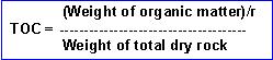
In the first place the wt% TOC must be related to the wt% kerogen. The ratio of TOC wt% to wt% organic matter is called "r" and will normally vary between 1.0 for an overmature SR to 1.5 for an immature SR.
The density of organic material (o varies from 0.9 to 1.05, depending on type of SR and maturity.
(1)and switching to organic matter:
 (2)
(2)
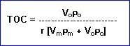
In the following the formulas will be simplified by using the following symbols:
Vb = Bulk rock volume
Vm = Matrix volume
Vo = Volume of organic material
Vf = Volume of fluids (water in porosity)
por = Porosity fraction
ρb = Bulk density
ρm = Matrix density
ρo = Organic matter density
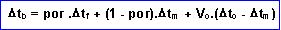
Then, considering volumes:
 (3)
(3)Simplifying:
 (4)
(4)Vm can be expresses as
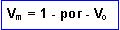 (5)
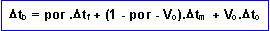
(5)Substituting this in (4) and solving for Vo gives:
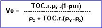 (^)
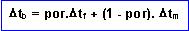
(^)The bulk density is:
 (7)
(7)or:
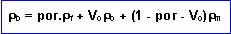 (8)
(8)Formulas (8) and the substitution (6) for Vo can show the effect on density of various contents of TOC. (Note that TOC in these formulas are fractions, not percentages).
Small changes in TOC have a surprising effect of on the bulk density. So, under ideal circumstances, the densilog should be a good tool to evaluate source rocks. Unfortunately, in practice, the densilog is affected by borehole roughness, measuring mud density rather than formation density (leading to over-estimation of TOC) in some cases, and presence of pyrite, which masks the effect of light organic material (under-estimation of TOC).
Density is partly determined by compaction. To estimate TOC the state of compaction must also be known, or eliminated in some way. The easiest way is to use a resistivity/density crossplot to circumvent measuring of the compaction state (Meyer & Nederlof, 1984).
Sonic log
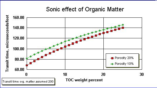
The sonic log gives the "slowness" (transit times) of the sound in terms of microseconds per foot, or microseconds per meter. This is usually indicated by Δt. The effect of organic material on the slowness is studied by assuming that it replaces matrix. One could also consider it as filling part of the pore space, but it is more convenient to group organic material with the also non-conductive mineral matrix.
Wylie's "time-average" formula is:
 (9)
(9)Having part of the solids as organic material, the time-average formula becomes:
 (10)
(10)or
 (11)
(11)where Δto is the slowness of the organic material. This is unknown, but likely to be on the order of 200 microseconds per foot.
The Δt is a function of porosity (compaction) and of depth (c.q. pressure). To estimate TOC, the state of compaction has to be known, as is the case for the use of the densilog. By using crossplots of transit time versus resistivity the state of compaction is eliminated. In practice, a multiple regression equation replaces the crossplot.
The above theoretical effects do not immediately provide a way to estimate TOC in practice. As mentioned above, the state of compaction is required as a basis for the estimate. We should know how far density or transit time deviates from that of a barren rock at the same state of compaction. There are various schemes to do this. Meyer & Nederlof (1984) used sonic and density/resistivity crossplots, but only give formulas for a simple classification into SR or non-SR. The method proposed by Passey et al. (1990) is probably one of the best, but requires making overlays of logs, scaled in a particular way as well as determining the maturity of the section in terms of LOM ("Level of Organic Metamorphism", which can be converted to approximate Vitrinite reflection values often abbreviated as "VR").
This program will be less accurate in estimating TOC than quite a few of the more elaborate methods proposed over the last decade and more locally calibrated, but is useful for a first screening of logs at least. It is based on world-wide data sets from literature where depth, TOC, resistivity, c.q. density was available. A multiple regression has provided two equations: one for the density/resistivity and one for the sonic/resistivity method. In essence, it is simply an extension of the Meyer & Nederlof (1984) method, but gives estimates of TOC instead of a simple classification into SR and non-SR on a fixed richness of 1.5% TOC.
In this method, rather than correcting the measured resistivity to a particular standard temperature, it uses the depth as a third variable that in a gross manner takes care of the temperature effect on resistivity. It also serves as an implied generalized campaction curve.
The data are from a very wide variety of areas and circumstances. Therefore the derived equations should be widely applicable, however, with the penalty that the accuracy will be low compared to the same method based on a local calibration.

The input sheet requires title information and the units for depth and transit time. Note that the depth units (meters or feet) and the slowness units (microseconds per meter or per foot) matter for the calculation! The user can specify the TOC cutoff value. If not, the program assumes 1.5% as a default value. The cutoff is important for a proper definition of net source rock for Gaea50 input. The log readings are entered in the table which allows 500 data to be entered. Both sonic and density readings can be entered or only sonic or only density. Resistivity is always required.
With "Files/Open" an existing input file can be entered into the program for correction or addition of data. The input can similarly saved for later use. The input files are textfiles with a single line for each data item. The first line is the title, the second gives the code for the depth units (True = Oil field units), the third is for the Sonic slowness units (Microsec/ft = 0, Microsec/M = 1). The following lines in the file contain Identification, Depth, Resistivity, Slowness, Density, which from the entries of the input grid.
The regression constants of this program are stored in the ...SourceLog\SourceLogData\SRLogBetas.txt file.
The Defaults for units are Meters for the depth units and Microseconds per foot for the sonic slowness.
The demo data are in ...\SourceLog\SourceLogDemos\*.txt files.
The results are shown in the same grid as the input. On the right is the estimate of TOC and then the Low (95%) and the High (5%) confidence limit. These three columns are first given for the sonic-based estimate, then for the density-based estimate.
This is a plot of TOC estimate versus depth, a kind of horizontal histogram with the depth scale on the vertical axis. The estimates are in red for the sonic/resistivity estimate and blue for the density/resistivity.


The histogram bars combine the the sonic and density-based estimates on the same histogram.

Carpentier,B., A.Y. Huc, G Bessereau (1990) Wireline logging and source rocks -- Estimation of organic carbon content by the carbolog method". The log analyst, S.P.W.L.A. Houston, 1990?) and in Revue de l'Institut Francais du Pétrole, v. 44, No. 6, p.699-719.
Meyer, B.L. & M.H. Nederlof (1984) "Identification of source rocks on wireline logs by density/resistivity and sonic transit time/resistivity crossplots". BAAPG v. 68,No.2, pp.121-129.
Passey, Q.R. et al.(1990) "A practical model for organic richness from porosity and resistivity logs". BAAPG, v. 74, No. 12, p.1777-1794.