Fieldsize distribution theories
It has been said that the lognormal distribution is in nature, and certainly in geology, more common than the normal distribution. The reasons are varied and worth a discussion about the possible mechanisms that would cause a skew, if not a precisely lognormal distribution of field sizes. But the fundamental question remains: Does nature allow a simple analytical description of fieldsizes in view of the complexity of the petroleum system? Probably not. Therefore the aim is to find an engineering solution, an experimental distribution, that can serve to make reasonable predictions. The danger lies in the attempts to extrapolate. There are a few well-known reasons why the observed data used may well be misleading:
- Definition of a play or province. How uniform is distribution of the set of fields sizes? Another definition of the boundary of the sampling area will give different results.
- Are the fieldsizes corrected for growth of Ultimate Recovery through appraisal?
- Bias in reporting only fields exceeding a certain economic size (cutoff).
- Effects of the creaming process. If there is a fundamental distribution law at all, would it not become visible only in an exploration-wise fully mature play? At that point, extrapolation or prediction becomes hardly relevant.
Multiplication process
By using a very simple model of fieldsizes, sometimes called the "Camembert model", referring to the well-known french cheese, consider three variables: productive area, net pay thickness and a factor comprising the "barrels per acrefoot" as a recovery factor. Now, regardless of the form of the individual distributions, their product will in most cases tend to a skew distribution that is somewhere in between a lognormal and a normal distribution. It would be more realistic to have a lognormal distribution of the productive area, as often is observed in basins. In that case the product would fit the lognormal much better. The theoretical consideration is that the multiplication of the three variates is equivalent to addition of their logarithms. For addition of independent variates the central limit theorem suggests a normal distribution for the result (in this case the logarithm of the reserves), hence the reserves would approximate a lognormal. We give an example with some hypothetical normal distributions for the three parameters.(See also a similar exercise with the throws of four dice).In a further experiment we consider 7 normal variates: length, width, gross reservoir, Net-To-Gross, porosity, oil saturation, recovery efficiency. Then with a Monte Carlo model that multiplies random draws of these 7 variates gives the following result:
 Normal fit is not accepted. |
 Lognormal gives a better fit, but far from perfect. |
The conclusion is that the multiplication principle is pointing to a lognormal distribution, but not the prime mechanism behind a lognormal field reserves distribution.
Breakage laws
When a rock is crushed and then the pieces are broken, and so on, the final distribution of the lengths of the pieces is very skew and can be described by an exponential distribution: the Rosin-Ramler Law . A similar skew distribution is observed for the size of meteorites (Frost, 1969) and for grainsize distributions.In the case of structural as well as stratigraphic traps, one may assume that there are centres (traps) that concentrate the migrating oil from the surrounding area. Such "drainage", or "fetch" areas are subdividing the whole area more or less in a random way. The size of these random drainage areas tends to a lognormal distribution. Here is an example of random polygons around centre points that are randomly distributed in the total area. The polygons are constructed by determining the midway point between neighbouring points and then drawing perpendicular lines through those midpoints. In practice the following map was created by a growth algorithm that grows ever wider layers around a nucleus, but not overwriting an element of a neighbour's layer. Each nucleus gets it's turn to grow.
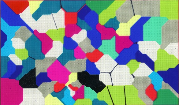
The size of the polygons was counted in pixels as an arbitrary area measure. Below is the goodness of fit test for the lognormal.
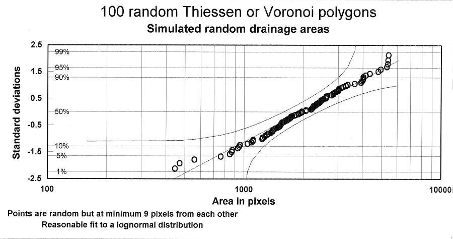
In a real situation these geometrical drainage areas are not equal to effective drainage areas, partly because of unequal presence of sourcerocks or degree of maturity. Such complicating factors are multiplicative and will enhancethe lognormal shape of a hydrocarbon charge distribution.
In the Gaeapas model a charge is calculated and a trap capacity. The model then accepts the minimum of the two volumes. Either the trap is full to spill (trap constraint) or the trap is underfilled (charge constraint). The trap capacity may also be constraint by top and lateral seal to complicate matters. An interesting consideration is that, a priori, the charge and trap are (more or less?) independent variates. Various arguments and data suggest that trap capacities are also lognormally distributed. Sometimes, in a geological play all traps are filled to spill. Then the distribution of trap capacities rules. But in plays where only part of the traps are filled, one should expect the mixture of two different lognormals, one for charge and one for trap.
Another complication is vertical stacking of reservoir/seal pairs. In the Niger Delta, Ultimate recovery is better correlated with, simply, the number of stacked, (independent) pools than with the productive acreage. Also the number of pools in fields is approximately lognormally distributed.
Conclusion:
Dictated by a skew, if not lognormal distribution of elements in the petroleum system, a skew fieldsize distribution is strongly suggested, but sometimes with a "dogleg" suggesting a mixture. The bias due to non-reporting of the smaller fieldsizes may mean that the underlying distribution is more like a Pareto, but the observed distribution more like lognormal (Hood & Sinding-Larsen, 2008). See also the study by Laherrčre (2000).