Geostatistics and Kriging
Many data used inprospect appraisal are distributed in an area. A common problem is to estimate , e.g. porosity, at a proposed drilling location, on the basis of data from nearby wells. Normally it is a problem of contouring, if at all possible. In our context we would like to know, not only the best estimate of porosity, but also the uncertainty, or variance. Geostatistical methods allow to find a best estimate and its variance. In this way we obtain an expectation curve of porosity for a given location. A fairly simple statistical principle is at the root of these methods.
First we consider that a random variable Z, measured at a location (X,Y) can have a probability distribution of some shape. This distribution is usually described by a mean and a variance and some analytical expression of the density curve ("pdf"). Assume that there are n locations (Xi,Yi) where a value Zi is measured.
Statistical theory tells us that the sum of two random variables has a variance equal to the sum of the variances of the individual random variables. Equally, but less obvious, the variance of the difference of two random variables is also the sum of the individual variances! This latter fact is used in geostatistics for a particular "local" variance estimation.
In our theoretical example of data Z on a map at various locations, we can measure a "local" estimate of the variance of Z, by calculating the squared difference of Zi - Zj.:
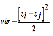
Here we assume that the two Z values are coming from the same distribution and have therefore the same mean value. The mean is cancelled by taking the difference of the two Z-values. This means that the we have squared deviations from the mean, and hence a variance estimate. We divide the squared difference by two, because we have the sum of two variances here and we only want the variance of Z.
By taking all the possible pairs of points on the map (i not equal to j) and making these calculations, estimates of the variance become available (�n(n-1) in number), which are associated with their point-interdistances. The results can be grouped in classes of interdistance "h". A plot of the variance versus h is called a "semi-variogram" or simply "variogram" (Clark & Harper, 2000, Delfiner, 2007).
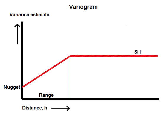
Taking the square root of the variance turns this graph into a standard deviation versus h graph and can be called a "sigmagram" (sigma is the Greek letter normally used to indicate a standard deviation of a population). This display has the advantage that the vertical scale is comparable to the scale of Z values and not the squared values. But note that the Kriging methods must use the variance values. Autocorrelation will show up on the sigmagram (and of course on the variogram as well) by having a cloud of points that have low standard deviation (c.q. variance) values at short distances. In the ideal case one sees a rising curve up to a certain height corresponding to the overall standard deviation of the variable Z in the whole area. The distance where the curve becomes horizontal and constant (the "sill") indicates the radius of the "zone of influence", shortly "range". Within that zone other points have something to tell about the value of Z at its center point.
It is often observed that the sigmagram does not start at zero variance at zero distance, but somewhere higher on the vertical axis. This is called the "nugget" effect. This would be normally caused by uncertainty of the measurements at the individual points. The values at distances greater than the above radius are essentially independent values. Clearly, prediction of the value at a point x,y should be done by using the k data points in the vicinity, i.e. within the zone of influence. One can imagine a linear relationship, such as:
where Zx,y is the required estimate, β the weight coefficient that is dependent on the distance h. These weights will be related to the inverse of the variance estimate at distance h, because that is a measure of the amount of information that the Zi value contributes to the value of Zx,y. The variogram can be modeled by various functions. In the following examples the function chosen is just a straight line from nugget to sill. The symbol "ε" stands for the uncertainty of the Z estimate. This can be quantified in such a way that not only a contour map of the variable Z can be made but also a map showing the standard deviation of Z. On such a standard deviation map there will be "lows" around the data points, because there the estimation is more precise than further away from the observed data points. In areas without data the standard deviation becomes roughly the "overall" standard deviation of the variable Z in the whole area.
A complication arises when there is anisotropy. This means that variograms differ when looking in different directions. In the examples discussed here we have omitted this aspect.
For a more complete explanation of the geostatistical techniques we recommend the book by Harbough et al. 1995, Chapter 7 and the electronic book by Clark and Harper (2000). A very good introduction is found at the Spatial analyst website, which shows the formulas required and discusses the various types of kriging. Also worth reading is the introductory article by Olea in Yarus & Chambers (1994), or the book: Olea, 1999).
Validity of contouring
The geostatistical theory can be used to check if contouring data on a map makes any sense at all. Here we give a figure with porosity data on a map that invites a geologist to start contouring it. He might spend a difficult ten minutes, or so, to realize that it is very difficult to make sense of the data. In fact these are random data at random positions. The variogram (300 points) shows that there is no autocorrelation of any significance. This is shown by a variogram that is horizontal at the sill value right from zero distance h till the maximum distance between points (horizontal red line). In other words: the nugget is equal to the sill.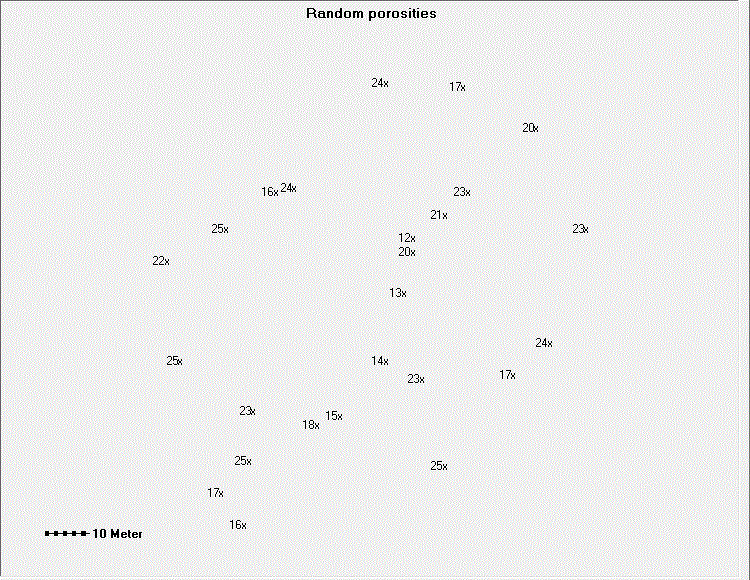
The variogram looks like this:
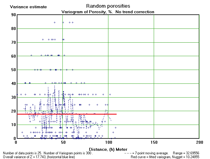
Here the zone of influence, if any, is at least smaller than the smallest interpoint distance. Contouring is always possible with geo-fantasy, but does not help!
A similar problem of estimation occurs for a one-dimensional series of data, e.g. log measurements. Can we interpolate intermediate values or would we be fooling ourselves?
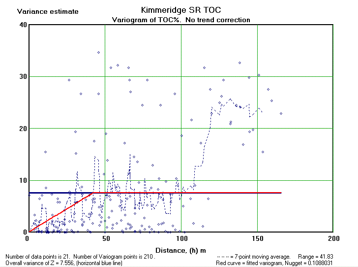
A variogram of one-dimensional data can give an insight. Here we have a variogram of 21 TOC (Total Organic Carbon) values measured in a well. The mean TOC value is about 7 %. The variance is 7.56. Interpoint distances vary from 3 to 166 meter depth. In this case the variogram suggests a range of 42 m and a negligable nugget of 0.1, or 1.4% of the variance. A clear case of autocorrelation that can be used to interpolate TOC values between the actual observations.
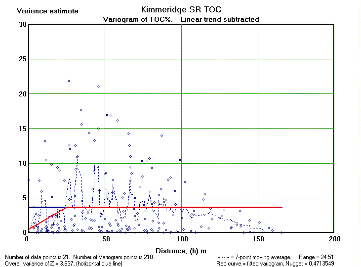
Hoewever, it may be that part of this autocorrelation is due to a trend in the data, the so-called drift. Therefore we repeat the analysis after substracting a linear trend. The trend of increasing TOC values upward proves to be statistically significant. The analysis uses the residuals from the linear trend for the analysis. Now the variance of TOC residuals is 3.64. The range is reduces to 25 meter, still indicating autocorrelation at a small scale and useful for interpolation of values. The nugget increased a little, but can be neglected.
Conditional simulation
In the previous section we have seen that a scheme can be devised to estimate data at any location (X,Y) and also to estimate the variance of Z at that location, taking the autocorrelation into account. An interesting application of this ability is to make not only one map of Z but a number of "equally likely maps" of Z, in a Monte Carlo fashion. This procedure is called "conditional simulation". A possible use of simulation is where seismic data are contoured and a closure is interpreted from this data. The uncertainties about the closure and it's size can be studied with conditional simulation, not generating a thousand maps, but perhaps ten or twenty, giving an idea of the uncertainties that can hardly be obtained by other means. A contour structure map of a suspected closure might show a valid closure of some of the equally likely maps, but not on others. In that way one could estimate the "probability of existence" of the closure.More elaborate use of this method is in simulating reservoir architecture.
The full theory of geostatistics is immensely complex. Here we have touched only on a few of the principles:
- The possibility to use data to construct a "sigmagram" with the purpose of checking on autocorrelation in the data. Note that this is just as valid and practical for data along a borehole (one-dimensional) as for data on maps (two-dimensional) and can be extended to three dimensions as well (e.g. mining or reservoir engineering).
- Use the range from the sigmagram, c.q. variogram, to see where data become independent from each other and use this information in sampling schemes.
- Use geostatistics programs ("kriging") to make estimates of the mean value and the standard deviation of a variable for a point on a map.
- Use geostatistics to simulate values on a map and study the uncertainty of those estimates by conditional simulation.