Addition of statistical variables
To evaluate a concession, play or a prospect with multiple objectives, etc. it may be required to calculate the sum of individual expectation curves. That process is addition, or aggregation. In other situations there may be more than one expectation curve for a single prospect/objective, because there are alternative evaluations made with different assumptions. The latter problem is one of merging.
The following problems deserve attention:
- Addition of distribution parameters
- Dependence of volume distributions
- Analytical versus Monte Carlo addition
- Combination of Probabilities of Success (POS)
- Merging alternative hypotheses
Note the difference between the P90 and P10 sums and between the P10 and P90 of the stochastic addition. Adding stochastically with independent expectation curves reduces the coefficient of variation (the standard deviation divided by the mean). That is reflected by the smaller difference between P90 and P10 for the last row of the table.
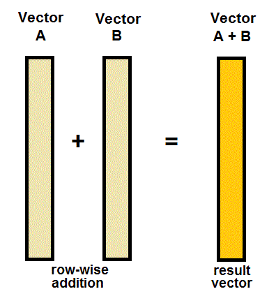
The procedure for a Monte Carlo addition is schematically given below. It may have to involve a "shake" subroutine to randomize the sequence of items in a vector. This can be done by creating another vector, filling it with random numbers between 0 and 1 (the RND function) and then sorting this vector while carrying the other vector along.
Dependence of distributions
Dependent prospects, or discoveries have volume expectation curves that are correlated to some extent. Under complete dependence, e.g. if Abel is turning out good after drilling, the other two will also be good, and if one of them is bad, all will be bad. Under independence and summation, a small outcome from Abel may be compensated by an above average outcome of the other two prospects. Then it has been shown that the variance of the sum of a number of a number of independent distributions is the sum of their respective variances (Bienaym�, 1853)
Dependence means, statistically, that there is non-zero covariance. Prospects in the same setting may have parts of their uncertainty (variance) in common. For instance if there is doubt about the sourcerock, this may be the case for all the prospects there. This effect is called here "commonality". For this reason it is useful if an appraisal system gives an analysis of variance ("ANOVA"). The results of such analysis helps in quantifying the covariances amongst prospects. For PSA approaches that specify the "Chances of Fulfillment" of a number of geological factors, it is usually assumed that these chance factors are indpendent.
An "addition program" should allow the user to introduce all the dependencies, possibly in a hierarchical fashion. The addition scheme is similar to the figure given for independent addition. In the dependent case, one of the vectors is arranged in order to create the right degree of dependence. See also the chapter on Monte Carlo methods.
Negative dependence
In prospect appraisal a negative dependence can occur if two prospects or targets fight for the same hydrocarbon charge. Imagine a single structure with two objective horizons, both to be charged by a deeper source rock. If there are doubts about the seal separating the two reservoirs and the charge is thought to be limited, we get an "either/or" situation: The upper reservoir wins if the seal covering his deeper competitor is bad, whilst the alternative is a lower target charged but the upper dry.
An interesting aspect of this example is that the geological commonality between the two reservoirs is negative, and dependent on ourbjudgment of the intervening seal.
In the above formula for the variance of the sum of dependent distributions, the third term is then substracted instead of added, due to the negative ρ. This results, of course, in a smaller final variance than in the above example. This can be explained by imagining two vectors of numbers A and B, as used in a MonteCarlo analysis. Negative correlation means then that relatively often a small value in A will be added to a large value in B. In positive correlation, large values in A will meet large values of B and causing a wider distribution range for A + B than in the negative ρ case.
A negative correlation can be simulated by partially sorting vector A in descending order, while sorting the corresponding part of vector B in ascending order.
The procedure to estimate dependence between two prospects cosists of:
A statistical estimate, based on ANOVA (Nederlof, 1997).
A geological adjustment of the statistical dependence through subjectively estimating the geological commonality.
The adjustment will, in general, reduce the statistical dependency estimate. The final dependency estimate is the correlation coefficient "r" of pairs of estimated distributions of volumes.
Another suggestion to estimate interdependence is the "kriging" approach. In that case the geological reasoning is less detailed than in the above method. The kriging logic is then that the success rate and/or size of the accumulations are spatially correlated. The zone of influence, or range, is used e.g. in the Gaea50 program for a bayesian update of P[HC] (probability of charge) based on the evidence from previous drilling. For interdependence the notion of spatial dependence has been used by Wees et al., 2006.
Usually a positive spatial correlation is observed for a parameter. If not the variance of the addition of estimates at different locations will be the sum of individual variances. The positive spatial correlation will increase it.
Addition of m = 2 distributions
How is dependence affecting the addition of distributions? For the mean value of the sum (Prospect 1 + Prospect 2) the addition is simply the sum of the means: Mean(1+2) = Mean1 + Mean2., regardless of the dependence.
For the variance with independence the variance of the sum is the sum of the individual variances:
 (1)
(1)With dependent prospects the "correlation" is involved. The dependence percentage in the above discussion is comparable to the R-square, the fraction of explained variance in a regression of Y on X. The square root of this is the "correlation coefficient". For prospects A and B with a correlation ρ, the variance of the sum is:
 (2)
(2)
For instance: prospect A has a mean (expectation) of 100 and prospect B 400 mb. The variance of A is 121 and that of B is 1296. The dependence (fraction) here is 0.40 (in terms of R-square), which means that we think that 40% of variance is common to the prospects A and B. This issimilar to estimating the R-square of a regression. However the formula requires the "correlation coefficient, which is more difficult to estimate than the R-square. (So ρ = 0.6325, the square root of 0.40).
Then the distribution of the sum A + B will be a distribution with a mean of 100 + 400 = 500 and a variance of approximately:
 (3)
(3)Note that in the case of total independence the variance of the sum would be 1417, the correlated example 1465 and in the case of complete dependence (100% or ρ = 1.0) it would be 1492.
Addition of m greater than 2 distributions
The above formulas can be extended from 2 to m distributions. note that the right part of the formula: 2*ρ*Sqrt(VARAVARB) actually is equivalent to 2*Covariance(A,B). We use the covariance matrix and then twice the sum of the covariances in the upper triangle, or what is the same: the sum of both the upper and lower triangle (off-diagonal) and omitting the factor 2. This is, of course the algebraic sum. It may be that some of the covariances are negative. These will reduce the variance of the addition result, while the positive covariances will increase it. In formulas:
 (4)
(4)
Example calculation of addition of m = 3 distributions
Here an example calculation, with positive and negative intercorrelation (interdependencies) of the three variables.
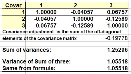
Three artificial distributions were used in this example. Two of the covariances are negative, and as mentioned before, positive covariances will be more common in practice.
The above rules for addition of correlated distributions, for instance, probabilistic estimates of reserves in prospects, it is important to know that the rules are valid for any kind of distribution. So, if you have lognormal estimates, you should calculate/estimate means, variances and covariances from the values as they come, i.e. not log-transformed to get a normal distribuion. A real example is my peak production estimates on te basis of a regression. The prediction is a regression equation: log(peak) = a + b*log(Ultimate Recovery), as the data are nicely lognormal. The R-square is 0.89. If the regression is calculated on the non-transformed data, it is 91%. Not a very large difference, but for other data it may well be larger.
From this high explained variance it is clear that the covariances between pairs of estimates are very high. In a Monte Carlo simulation adding such estimates, we would calculate the variances of each estimate and derive the covariance for a pair from the right side of formula (2) above. The correlation coefficient would be in the example the root of 0.91, or about 0.95. Clearly a case with a very strong dependence, because all the estimates are based on the same regression equation.
Unrisked Sum. Although the above calculation can be done by hand, the "unrisked" sum of prospects requires a Monte Carlo addition, including the correlation, whereby in each cycle a prospect resource is added to the total, but only if the binomial simulation of its POS is 1. For the Mean Success Volume again a hand calculation might suffice, provided we have the means of the unrisked volumes of the prospects available. The each mean is multiplied by its POS and added to the sum.
Addition of expectation curves by analytical means is sometimes possible if the distributions can be expressed in mathematical form. Even then, the maths may become complicated. In many situations, the distributions to be summed do not behave well enough for a mathematical addition. Also, explaining the Monte Carlo procedure is often easier than explaining the rather complicated analytical procedures. Some decades ago, computer resources limited the use of MC procedures. Now, however, this does not appear to play a significant role.
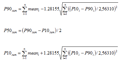
However, it may happen that to aggregate only a table with the percentiles for a set of discoveries is available. If the P90, P50, Mean and P10 are available, the following shortcut avoids the Monte Carlo addition procedure, but only gives the result under assumption of complete independence. The sum of a set of distributions has a mean equal to the sum of the individual means. Also, provided thet the prospects are not dependent, the variance of the total is the sum of the variances. So, for each prospect we estimate the variance from the difference between the P10 and the P90 in terms of a standard deviation. For a normal distribution the (P10 - P90) = 2.56310 st. deviations. If the individual prospects show a lognormal distribution, the same formula holds, but then (LN(P10) - Ln(P90)) = 2.56310 st. deviations (as logaritms). Here are the formulas for both cases.
The normal distribution case for the sum of n distributions, where the mean of the sum is the sum of the means, but the percentiles are:
Analytical versus Monte Carlo addition
For the lognormal distributions the distribution of the sum is probably neither lognormal, nor normal. But we could use both models, realizing that the reality will be somewhere in between. The larger n, the better the sum distribution will approach the normal. The procedure is here more complicated as we need to estimate the linear variance of the individual distributions, which is not so straightforward as in the normal case. Note also that the mean of the lognormal (as logs) is the log of the P50.

In the above formula "ln" stands for natural logarithm to the base e. The " * " is the multiplication symbol because the formula is too long for one line. Having the list of individual variances, the variance of the sum is the sum of the individual variances. We take the square root of this to get the standard deviation. Under the assumption that the sum distribution is approximately normal we can follow the same procedure to obtain the percentiles as explained above for the sum of normal distributions. (As is usual with logs, your math will blow up if any of the input numbers is zero!). Did I not tell you that the analytical procedures with lognormal distributions is complicated?
The above shortcuts are based on the assumption that individual distributions do have the shape of a normal or lognormal. If there is risk in the form of many zero elements in the distribution (exploration prospect) than addition is statistically unsound because of the distribution shapes, and, the addition of the non-risked P90, P50, P10 meaningless and misleading. In the risk case only add the expectations! And use a Monte Carlo system if the whole sum-distribution is required.
The above formula becomes simpler if we have equal probabilities of success for all n prospects:
Above we have assumed independent prospects. For completely dependent prospects the result would be:
See also Rose (2001, Appendix D) for a few more examples. By the way, In a Monte Carlo Addition complete vectors of possible reserve volumes, including the zeros are added together with various degrees of dependence. The final POS can then be read from the sorted vector of the result, this being the expectation curve of the sum. In that case the POS calculations as above are not necessary.
Effect of correlation (dependence) on the POS of the sum of prospects.
When the prospects have full dependence, the POS of the sum (POSDependent) will be equal to the maximum POS in the prospect set.
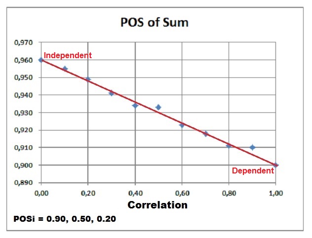
In case of complete independence of the prospects, the maximum combined POS (POSIndependent) is reached. In between these two extremes we can interpolate between these values in a linear manner, using the correlation coefficient r. Note that the POSIndependent >= POSDependent in all cases.
In formulas:
For 100% dependent prospects (r = 1.0) the "POSdep" of the sum becomes:

For the independent prospects (r = 0.0) the "POSind of the sum becomes:

For any r the formula is:

That the difference between the dependent and independent case is proportional with r can be demonstrated with the following Monte Carlo result, in which three prospects were summed with the individual POS's as indicated below the graph, of which 0.90 is the maximum:
Merging of expectation curves
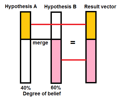
When there are two different, alternative appraisals made, a unique solution has to be found, unless decision making can handle such conflicting advice. It may be that the interpretation of a seismic section leaves so much doubt about the nature of a trap, that different possibilities are evaluated. Each alternative interpretation is then internally consistent. Combining this situation to form a single expectation curve requires that we assign a "degree of belief"to hypothesis A and to B. The degrees of belief should add to 100 %.
The merge process is as follows:
The Gaeatools program MAD (Merging and Addition of distributions) allows addition with user-defined degrees of dependence (covariance). It allows a hierarchical input of expectation curves.