Pareto Distribution
A line appears on a log-log plot. One hears shouts of "Zipf!","power-law!","Pareto"! Well, which one is it? The answer is that it's quite possibly all three. Let's try to disentangle some of the confusion surrounding these matters and then tie it all back neatly together.
Lada A. Adamic, 2002.
The Pareto distribution is also known as Zipf's law, Power-law density and fractal probability distribution. George Kingsley Zipf (1902-1950) studied comparative linguistics. Amongst other linguistic data, he found that the frequency of words occurring in text when plotted on double-logarithmic paper usually gives a straight line with a slope of -1/2 or, if ranks are used, a slope of -1. Zipf found that data, such as the size of towns, countries, concentrations of metals, etc, followed this rule, which become known as "Zipf's Law". For a discussion of the similarities/equivalence of Pareto, Zipf and Power we refer to Adamic & Huberman (2002). We could try to see whether oil field sizes also behave according to this, or similar laws:
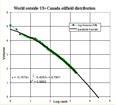
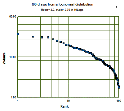
This graph, adapted from Khebab (2006) shows the pareto-type plot of log(reserves, 0 = one million barrels) versus Log(rank). The data are 2092 of the largest field sizes, i.e. larger than 50 million barrels. A parabolic fit has to be made, although a straight downsloping line might cover the largest fields of this set. In this first part the slope is close to -1/2, but toward the smaller sizes the slope becomes even larger than -1.0, on average -1.0. Is this really the underlying model of fieldsizes? As a comparison we did an experiment, generating 100 random draws from a lognormal distribution. The result on the log(reserves) vs. log(rank) shows a marked similarity to the previous plot by Khebab. Here also the slope for the largest fields is about -1/2, but on average -1.0. We do not obtain a straight line and hence the simplicity is lost, while the lognormal gives at least a straight line. See also the examples at the bottom of this page.
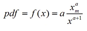
The pareto distribution is a continuous distribution with two parameters: a minimum value and an exponent. (The Zipf distribution is the discrete counterpart of Pareto). The probability density function is:
and the cdf as an expectation curve is:
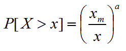
Conveniently, when we take logarithms we obtain:

This means that this complement of the cdf should form a straight line on a double logarithmic plot. With the probability on the Y-axis and the reserves on the X-axis the line slopes down to the right.
The mean is:

Note that a > 1, because division by zero is forbidden and a negative mean is impossible for a distribution of non-zero numbers.
and the variance is:
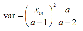
The variance does not exist if a <= 2, to avoid dividing by zero and to avoid a negative variance.
To apply the pareto, or similar distributions to fieldsizes is possibly an unnecesary complication. I let the reader decide after studying the following graphs. The following plot is a sample of 52 fieldsizes of Siberian gasfields, plotted on double-logarithmic paper.
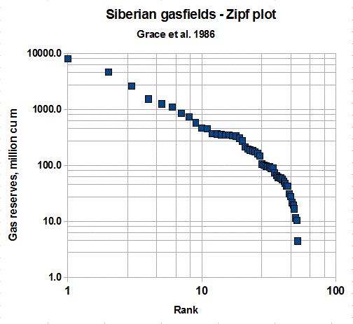
Here again the straight line does not appear. A parabolic fit to the curve would require at least three parameters. An almost perfect lognormal fit would only require a two-parameter distribution:
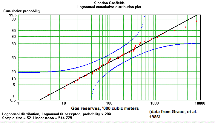
The goodness of fit test for the lognormal shows that there is no reason to try another distribution type for this sample.
However, when describing natural fractures, a power law distribution appears to fit better to the data than an exponential, or lognormal (Santos, 2015).