Helpfile for Prodcasting

General

Prodcasting is a probabilistic model for estimating total production to be expected from a number of new discoveries.
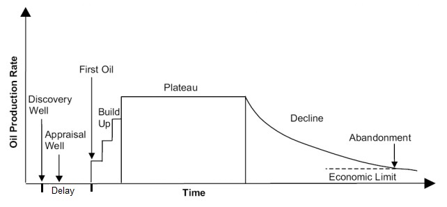
It needs a set of Mean success volumes after cutoff, the probability of success (after cutoff), and an assumption about the rate of exploration. Then for each modeled discovery a production profile is created and the profile added to the total in the corresponding years. The result is a set of scenarios in the form of a table and as a graph. The whole scheme of the production life of an accumulation is shown in the figure below:

There are three ways to define the order in which the prospects are supposed to be drilled:

1. Original input order, which may not be optimal.
2. Expectation rank,
   optimal in a way to obtain the maximum discovery early.
3. Random order. The original input is "shaken" into a random order.

Input

• Administrative input
• The prospects
• The settings

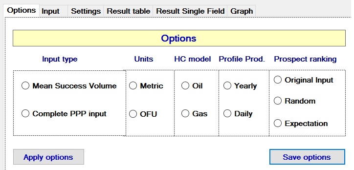
Administrative The administrative input comprises a general title to identify the modeling. The units are required to label the output tables and graphs. The input filename is not an input but shows which file has been opened, if an existing input was opened.

Prospects. The prospect input in the simple option consists of:

1. Prospect/accumulation name
2. Probability of Success after cutoff ("POSc"), %.
3. Mean success volume after cutoff ("MSVc"), "units".

Under the "Complete PPP input" the following data have to be provided as well.

1. The P90 of the Unrisked Success Volume distribution.
2. The P50 of the Unrisked Success Volume distribution.
3. The P10 of the Unrisked Success Volume distribution.
4. The distribution type of the Unrisked Success Volume distribution.

Note that the mean (MSV) in the PPPinput case , as well as the expectation is calculated by the program. The distribution types are: Normal, Triangular, Lognormal, Rectangular and Constant. For the triangular case the three parameters are the Low, Mode and High.
For convenience, a default type of distribution can be inserted in the Distribution type column, using the listbox above the input form, but only after the prospect input in the other required columns has been made.

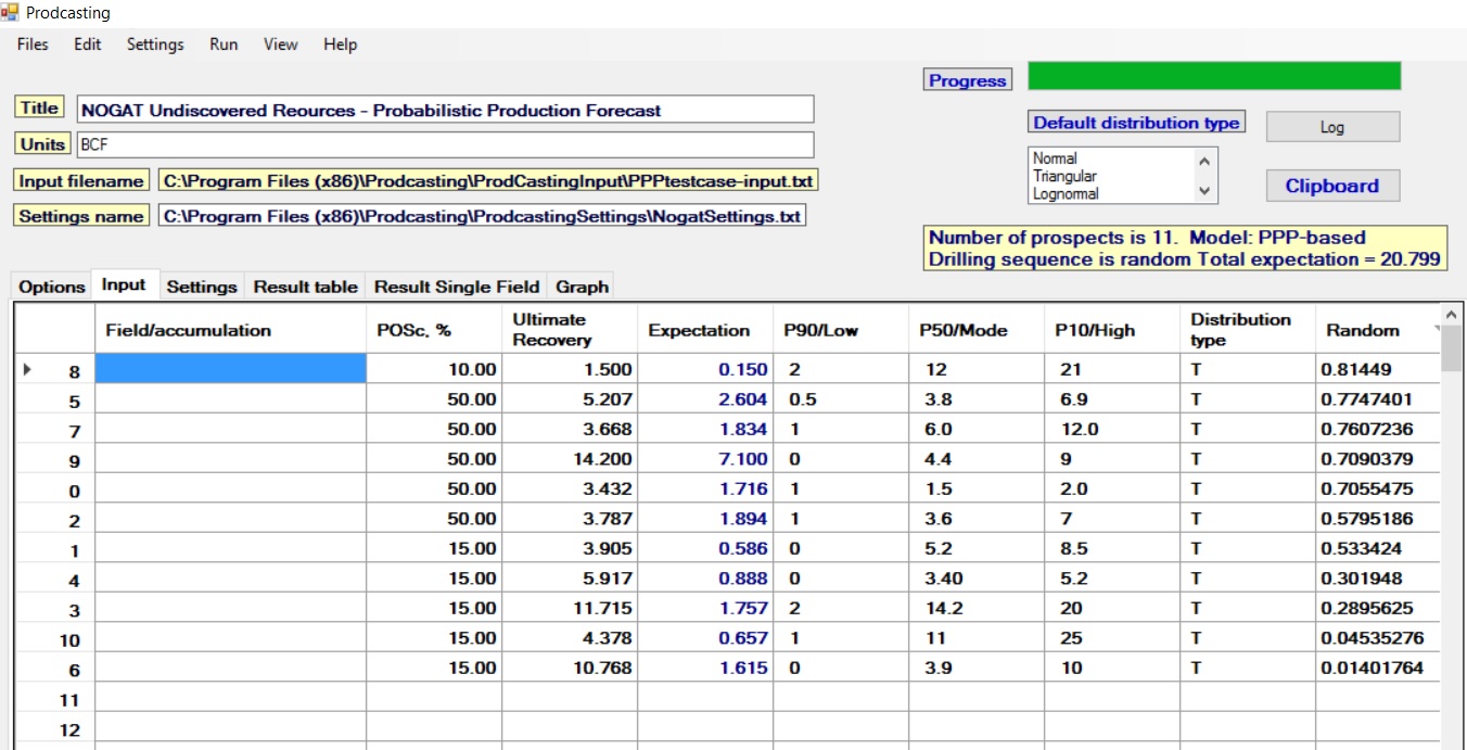
Note that the expectations are calculated by the program as MSV * POS, and do not need to be given by the user. In the above example, the option of sorting on expectation was used. The original sequence had an alphabetical order for the prospect list.
The MSV and POS values can be obtained from the AddRes output or other sources.

Settings. The settings are first of all a start year for the modeling and an end year.
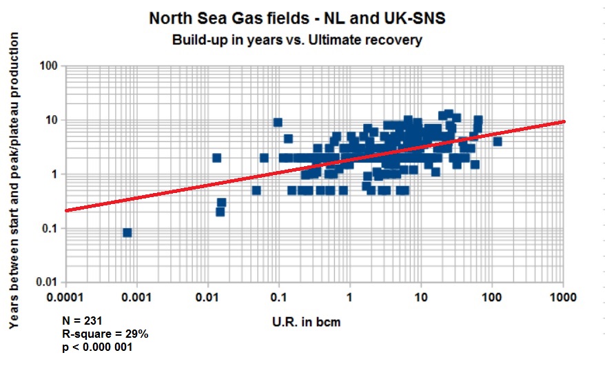
Other settings refer to the production forecast sub-model to estimate the profile for a single discovery. The individual discovery production profiles are modeled after, for an area with known fields, a number of factors have been statistically evaluated. Notably, the peak production is a function of the ultimate recovery. This generally holds for oil as well as gas over a wide range of magnitudes. Here we do not use the depth of the objective, which might influence the production rate of wells, nor the size of the field, which would influence the number of wells required and the speed of buildup.
The gas settings are the following:

1. Duration
1. Start year
2. End year
2. Peak/plateau production regression equation
   Estimating the peak production from the MSVc.
1. Constant (intercept)
2. Slope
3. Standard error of the residuals
4. Mean X
5. Standard deviation of X
6. Sample size of the regression
3. Buildup regression equation
   Estimating the years to plateau/peak from the MSVc
1. Constant (intercept)
2. Slope
3. Standard error of the residuals
4. Mean X
5. Standard deviation of X
6. Sample size of the regression
4. Decline % regression of log10(decline%) on Log10(UR)
   
   1. Constant (intercept)
   2. Slope
   3. Standard error of the residuals
   4. Mean X
   5. Standard deviation of X
   6. Sample size of the regression
5. Number of plateau years regression of plateau years on Log10(UR).
   
1. Constant (intercept)
2. Slope
3. Standard error of the residuals
4. Mean X
5. Standard deviation of X
6. Sample size of the regression
6. Number of exploration wells per year
   For less than one well per year, the input should be a negative integer.
   So: one well per three years would be "-3".
7. Average delay between discovery and frist production, years
8. Number of scenarios (maximum 10,000, default 100).

For oil the settings are the same for peak production and build-up years, but the decline % and duration of plateau production are represented by Low, Mode and High prior values as a triangular distribution.

Method

• Discovery process
• Single field forecast

Discovery process. This creates a number of discovery scenarios by drilling the specified number of exploration wells per year. As the prospects are not equally attractive, it is assumed that the drilling sequence follows an optimal order, based on a ranking of the risked means (= expectations). The drilling sequence may, for various reasons, be less than optimal. However it is not possible to foresee in how far it will deviate from the optimal. In a Monte Carlo simulation the wells are drilled and a discovery is made if a random number between 0 and 1 happens to be less than the POSc of the prospect, which is a binomial modeling. At this point the second simulation unit is invoked which estimates a volume of recoverable hydrocarbons and a production forecast made for this particular field's MSVc.

TRhe various regression equations and the associated parameters allow to make random draws of the four variables used to create a production profile in the Monte Carlo procedure. The calculation of the profile of a field for the length of the scenario and including a tail end beyond that till abandonement, may result in a total cumulative production that deviates from the MSVc. The expectation of the cumulative production + tail should be equal to the expectation for the prospect. The program adjust the results, using the total expectation of all prospects.

If the complete PPP input is given the MSVc is replaced by a single random draw of the ditribution determined by the P90,P50, P10 and the distribution type code. This is a more realistic approach and increases the final uncertainty of the production forecast.

The production profile generated for the single discovery is added to the grand total profile for all the discoveries, but shifted to the correct year of discovery.

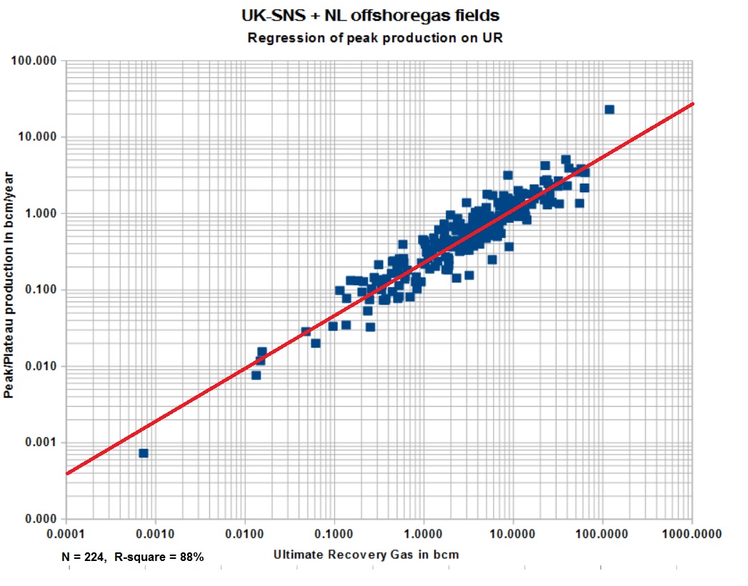
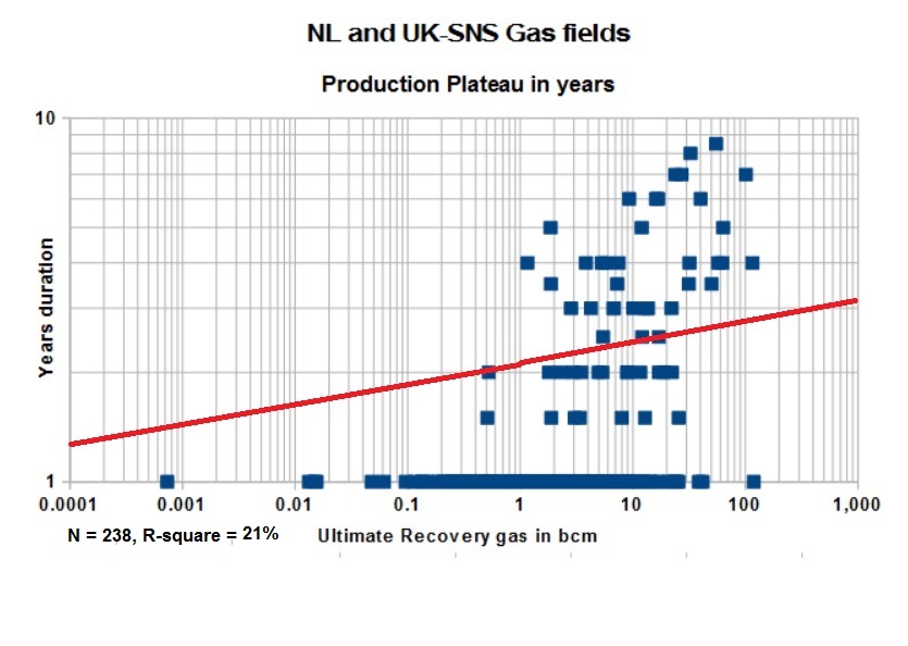
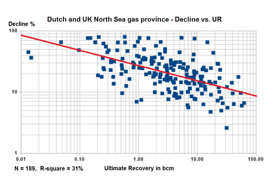
Single field forecast. The production profile is based on reasearch that established a relationship between the peak (or plateau) production and the Ultimate Recovery. Strong correlations were established for oil fields (r = 0.942) as well as for gas fields. Similarly the duration of the build-up phase is correlated with the U.R., but weaker. Both these regression results are stored, in principle, in the settings of the program. For the profile other variables are significant: the decline % after the peak and the volume produced till the end ot the peak and the duration of the plateau.

As examples of the relationships found the following graphs (one for gas, another for oil) may illustrate that a reasonable probabilistic automatic modeling is possible. The correlations found comprise the Peak/plateau production rate, the build-up years to the peak, the length of the plateau in years and the decline%, all regressions on the ultimate recovery.

The relationship between build-up years and U.R. is weaker (0.712), as shown below. Nevertheless it useful in the modeling.

The decline correlation for gas is also reasonable in the gasfields of the Netherlands offshore, combined with the many gas fields in the southern North Sea UK.

Results

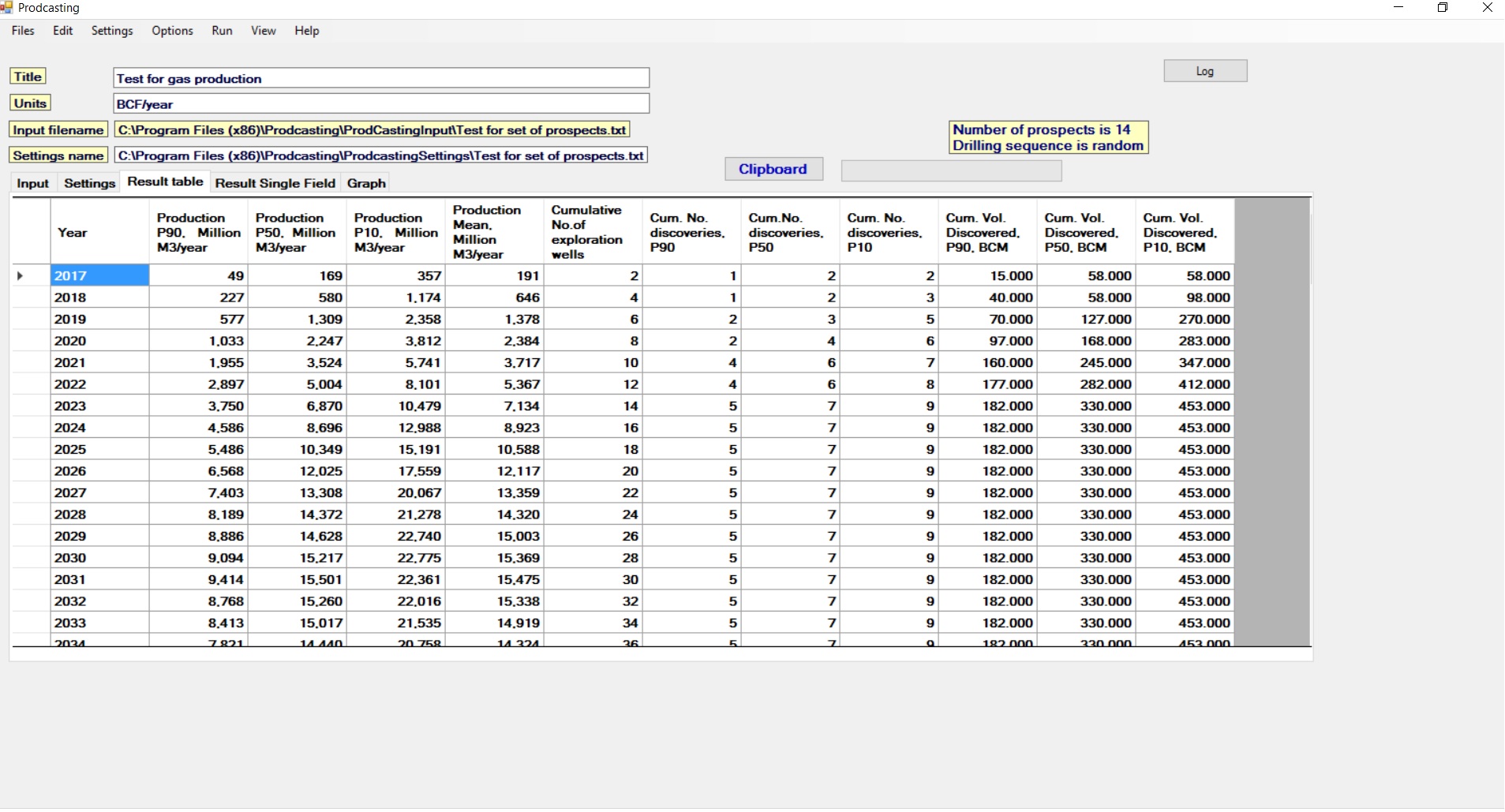
The result table shows the percentiles of production for the years of the scenario. In the above example, the simple MSVc input was used and the delay was 0 years.
The Clipboard button allows the copying of the whole table for e.g. pasting into a spreadsheet. This does not work for the graph.

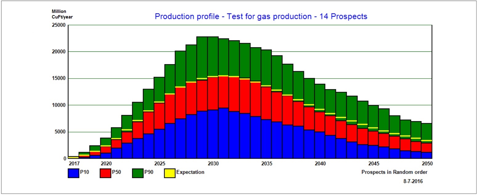
The production profile is shown as a graph:

• ProdcastingInput
• ProdcastingDemos
• ProdcastingSettings
• ProdcastingHelp
• ProdcastingOutput

Print