Triangular Distribution
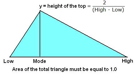
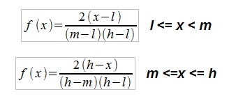
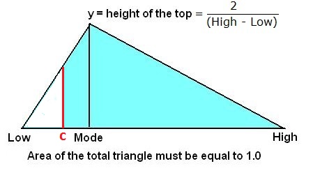
The triangular distribution is a useful tool if a variable has to be estimated subjectively. The estimator has to indicate a Low, a Most Likely value (Mode) and a High value, the distribution contained within the Low to High range. In the formulas below "l" is the Low, "m" is the mode and "h" the High value. In other descriptions (Wikipedia) the characters "a", "c" and "b" are used resp. for l, m and h. The pdf is a triangle:
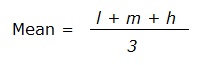
The mean is:
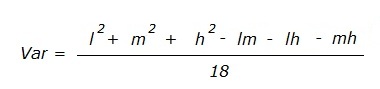
The variance is:
The CDF consists of two curved line segments, with a discontinuity at the mode.
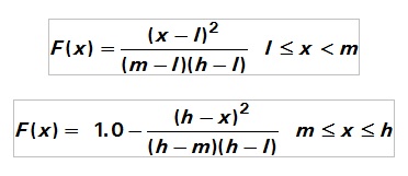
In this case it is interesting to know also the inverse form of the cumulative distribution function:
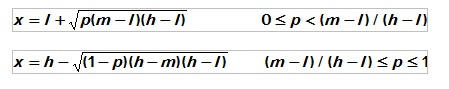
This formula is used in generating a random triangular deviate from a rectangular one between 0 and 1 in Monte Carlo analysis.
Mode estimator
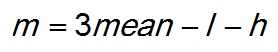
The triangular distribution can be fitted to a data sample to find a rough estimate of the mode. If the distribution type is unknown it is quite difficult to estimate the mode, as no simple analytical solution is at hand. In such case an easy way is to fit a triangular to the data by recording the lowest and the highest values as l and h, as well as calculating the mean. Then the mode (m) is:
Im practice, this estimate is very sensitive to the input parameters and in the Monte Carlo analysis I use a different method to estimate the mode. In a sorted vector X 21 percentiles are extracted. Then the midpoint of the shortest of these 5% percentile intervals is chosen. Arbitrarily, the mean of this interval is assumed to a reasonable estimate of the mode of a unimodal distribution. Note: Only used for estimating the mode in an unrisked vector. A risked vector has a number of zero values, a first mode, then somewhere to the right a mode of the non-zero values, hence not unimodal.
In prospect appraisal, it is sometimes useful to describe an unrisked volume distribution as a triangular. When an economic minimum volume is given, the original triangular will become truncated from the left, at a cutoff-volume "c". Then the MSVc, i.e. the mean success volume after cutoff has to be calculated. Also the POSc, or the probability of success after cutoff is required. The latter is the total risk: geological POSg + the risk to find HC, but less than the cutoff. These parameter, and their product (Ec = POSc times MSVc) can be analytically calculated.
Left-truncated triangular distribution
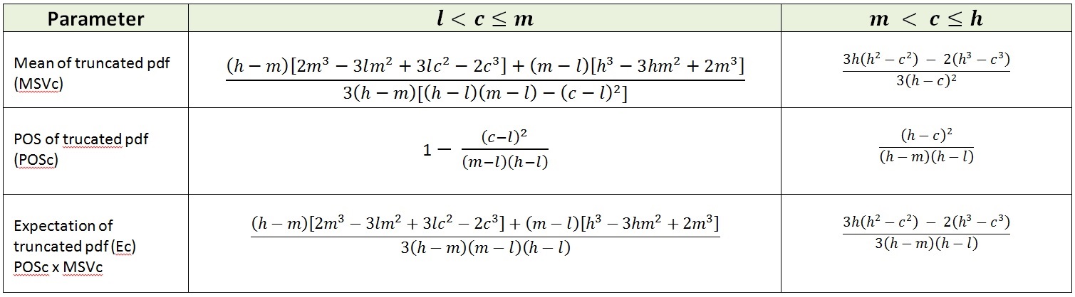
Probability to find less than the mean.
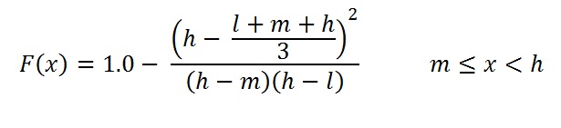
With prospect estimates, the mean is often larger than the median and this in turn larger than the mode (m). It is interesting to realize how much of the area under the density curve lies to the left of the mean. In other words: what is the chance to find less than the mean, given l, m and h of the distribution.
As we know the formula for the mean, we can substitute this in the formula for the F(x), the cumulative diostribution. Then we get:
To get a feel what this means, a "standard model" for the uncertainty of a volume estimate can be constructed by assuming that the mode m is 1.0, and then derive the low (parameter "l") by dividing 1.0 by a constant f and the high parameter "h" as f itself. Then the formula for the cumulative probability at the mean will be:
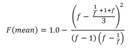
For f = 3.0 the result = 54.6 %. This factor gives a reasonable model for exploration prospects in the case of unrisked volume estimates. And, of course, for f = 1.0 there is no uncertainty (l = m = h = 1.0), the estimate is a constant. For a symmetric triangular distribution, the cumulative probability at the mean is 50%, because then the mean, the median and the mode will coincide at the same x-value.
In a more general case with the parameters 2,5,11, the area to the left of the mean (6) = 53.70 %. The most extreme case is one that has l = m , hence only the right triangular part of the distribution between m and h, which must have an area equal to one. A little algebra shows that the percentage, regardless of m or h, will be 1 - 4/9, or ~0.5555556 in this extreme case.