The beta distribution
and deriving a posterior probability of success,
When prospect appraisal has to be done in less-explored areas, the local known instances may not give enough confidence in estimating probabilities of the events that matter, such as probability of hydrocarbon charge, probability of retention, etc. Intuitively, one would seek to include experience from other , better explored areas, where probabilities have been established from a counting of a sufficient number of well-documented cases. If one has assembled such information the problem then becomes to combine this background information with a few local cases.
The above problem is one in bayesian statistics and can be reasonably solved by the use of the beta distribution. The reader is probably familiar with the binomial distribution, describing the uncertainty of a "Bernouilly"process. The unknown parameter is the number of successes "r" in "n" trials. The beta distribution focuses also on this sampling experiment, but considers the probability of success in a single Bernouilly trial as the unknown parameter. Its density distribution is:
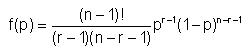
We use here a version of the beta distribution that is convenient for the discussion of "updating" the parameters by new information. Often you will find a slightly different formula, that involves the parameters α and β, respectively meaning r and n - r, in other words: successes and failures.
The mean of this distribution is:

Note that, if r is not equal to n - r, the probability density is skewed. The mode is:
and the variance is
The parameters r and n have a simple interpretation: n is representing the "equivalent" number of trials while r represents the "equivalent" number of successes amongst those trials. With n = 5 and r = 3 the pdf looks like this:
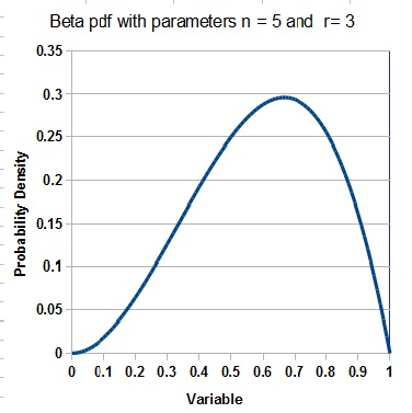
The mean = 0.600 and the mode is (3 - 1) / (5 - 2) = 2 / 3 = 0.667...
The beta distribution is used to describe the worldwide background experience as a so-called "prior" distribution with parameters r' and n'. The sample of cases in the local area of interest gives r sucesses in n trials. (Note that the "local" sample parameters n and r are written without primes!). If one did not have this local information, only the worldwide background information would be used, i.e. the required probability would be estimated to be r'/n'. On the other hand, if we had totally explored a certain area with n prospects, we would be sure of the local success rate. In that area we then sampled all n possible cases finding, say r successes. We would conclude that the probability is r/n. The prior information has become irrelevant in this case. In practice we will often find ourselves in between these two extreme cases. The scarce local sample information has to be combined with the prior information.
The bayesian theory allows the combination of the local information with the prior into a "posterior" distribution with parameters r" and n" (note the double primes to undicate the posterior parameters). The relationship between prior, local and posterior is given by:
So a simple addition of the parameters of the prior and the local sample gives the required result. The required probability is then r"/n".
There has been considerable discussion amongst statisticians about what represents the prior state of complete ignorance. From the above formulas used to update a prior to a posterior it appears logical to say that a so-called "diffuse" prior, containing no previous information, is a beta distribution with parameters r'=n'=0. This condition would nicely let the local sample results prevail in all cases, also in the extreme one mentioned above, where exploration has been completed and the local r and n are perfectly known. In practice, r' and n' are probably not equal to zero, but become gradually less influential in estimating the local probability with increasing local r and n. In practice, complete ignorance is unlikely and some data can be collected to estimate a prior beta distribution, i.e. r' and n'. The following example may illustrate this.
Example:
In 10 well-explored plays, the probability of hydrocarbon charge has been observed. In the counting
process some wells drilled are excluded, for instance a well clearly drilled off-structure. In a field with a
number of wells, only one of the wells is included. Within each play some of the tested closures did not
have hydrocarbon charge, possibly due to a number of geological causes, as distinct from technical reasons. Such plays form the
worldwide background experience telling us what to expect for a closure in our local play area.
For
Gaeapas, the counting involved some 330 “plays” or “provinces”, which on average are about 8000
square kilometers. A kriging exercise involving these areas involving some 30,000 exploration wells,
suggested a zone of influence of 50 KM. Here, as an illustration we give a selction of ten plays that mimic
the actual global distribution of p[HC]. The ten plays have provided the following estimates of the
probability for a single closure to receive a hydrocarbon charge : p[HC].
| Play | p[HC] |
|---|---|
| 1 | 0.04 |
| 2 | 0.12 |
| 3 | 0.20 |
| 4 | 0.20 |
| 5 | 0.30 |
| 6 | 0.35 |
| 7 | 0.40 |
| 8 | 0.50 |
| 9 | 0.68 |
| 10 | 0.86 |
From this table the following conclusions are drawn:
the mean of p(HC) = 0.365, or 36.5%
the variance of p[HC] = 0.058825
the standard deviation of p[HC] = 0.2425
The prior parameters are derived by using the mean and the variance
to estimate r' and n':
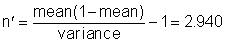
Note that a rather large number of trials have been counted in the ten plays, but this is not reflected in the "equivalent " number of trials n'. The widely varying conditions that one may apparently encounter over a number of plays has made the prior information equivalent to one sample of about 3 trials of which 1.25 are successes.
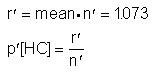
The process of "updating" the prior is illustrated by the following example. Assume that the local count shows two charge cases in three drilled closures. While the local ("sample") estimate of p[HC] would become 0.667, the suggested bayesian estimate would be:
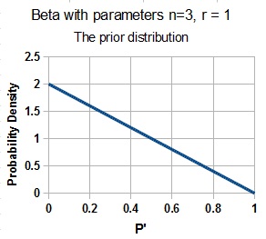
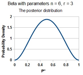
As an illustration we show the corresponding beta distributions with n' = 3 and r' = 1 ( the prior, and I have rounded the numbers for convenience sake) which is a triangular distribution with these numbers, and the posterior beta with n" = ~6 and r" = ~3, which resembles a symmetric, normal distribution:
 |
 |
This estimate is significantly lower than the two out of three chance suggested locally on the very limited information. If, however, the local count had been 20 successes out of 30 trials, the posterior probability would have become p"[HC] = 0.640, much closer to the estimate based on local data only. This is because the local information has then overwhelmed the rather weak prior information.