Monte Carlo Methods
- Analytical versus Monte Carlo
- Pseudo random numbers
- Generating analytical distributions in MC
- Latin square hypercube sampling
- Prediction based on a regression equation
- Simulating correlation between MC vectors
- Accuracy of Monte Carlo simulations
- Imagine a regression of Y on X as follows:
-
If we change to standardized variables (i.e. substract the mean and divide by the standard deviation) we denote the standardized X as a lower case x.
y = r.x + ε
Note that the intercept is now zero and the slope is simply equal to r.
-
For ε, the scatter, or noise, around the regression line, we generate a new vector of standard normal random numbers N(0,1).
-
Now we create a vector of regression estimates of y for each x. That is the regression result plus the noise that is the standard deviation of the residuals:

-
The vector y is now sorted carrying the original vector X along. Now X is in the correlated order with respect to the created vector y.
- Sort the complete original vector Y in ascending order. The correlation of vectors X and Y is established.
Experiments show that any required r can be modeled in this way with great precision.
- For subsequent use, the vectors should not be "shaken" individually, but in tandem, otherwise the correlation would be lost.
Here is a scatter graph from a MC simulation of 100 cycles.
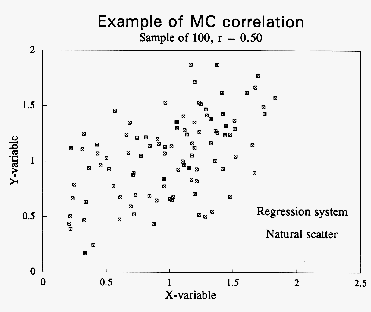
In the context of aggregation of reserve estimates we may have to deal with more than two vectors. In those cases the vectors that have the same dependence are treated in the above way. Other vectors (prospects) with a different interdependence are separately summed, after which the sums of groups are summed to the grand total. Within a group of 4 prospect with degree of dependence r the correlation matrix would look like follows:
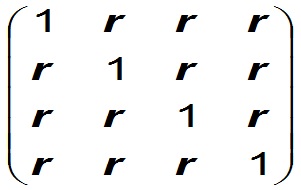
If, for some reason, a correlation matrix with several different intercorrelations would be required, a more sophisticated statistical method would be required (Haugh, M., 2004).
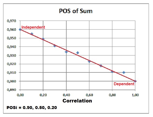
Effect of correlation (dependence) on the POS of the sum of prospects.
When the prospects have full dependence, the POS of the sum (POSDependent) will be equal to the maximum POS in the prospect set. In case of complete independence of the prospects, the maximum POS (POSIndependent) is reached. In between these two extremes we can interpolate between these values in a linear manner, using the correlation coefficient r. Note that the POSIndependent >= POSDependent in all cases.
In formulas:For 100% dependent prospects (r = 1.0) the "POSdep" of the sum becomes:

For the independent prospects (r = 0.0) the "POSind of the sum becomes:

For any r the formula is:

That the difference between the dependent and independent case is proportional with r can be seen in the following Monte Carlo result, in which three prospects were summed with the individual POS's as indicated below the graph, of which 0.90 is the maximum:
Unrisked Sum. Although the above calculation can be done by hand, the of the "unrisked" sum of prospects requires a Monte Carlo addition, including the correlation, whereby in each cycle a prospect resource is added to the total, but only if the binomial simulation of its POS is 1. For the Mean Success Volume again a hand calculation might suffice, provided we have the means of the unrisked volumes of the prospects available. The each mean is multiplied by its POS and added to the sum.
Accuracy of the Monte Carlo simulation results
The Monte Carlo process is never exact, unless with an infinite number of computation cycles. To see what the accuracy is, given a practical, finite number of cycles, a few simple statistical rules can be used. The expectation curve produced by the simulation represents the mean of Ncyc individual expectation curves, one for each MC cycle. The final expectation curve has a standard deviation. To get the standard deviation of the mean (expectation) we can divide this simply by the square root of the number of cycles used, as we may assume that the MC error is distributed normally for such a large sample.

Here n is the number of Monte Carlo cycles.
Similar rules are used for probabilities (POS), using the binomial distribution. If not too skewed, the binomial can be approximated by the normal distribution, especially in this context, with many MC cycles (= large samples). For an estimate of POS derived from n Monte Carlo cycles, its standard deviation (s is given by the following formula.
Here is an example of confidence ranges from the prospect appraisal program Gaeapas with 1000 MC cycles.

If the number of MC cycles is small in comparison with the uncertainties from the analysis, it may be that the calculated confidence limits at the lower end become less than zero. In that case the lower confidence must be set to zero. At the upper end, for POS, the 95% limit may exceed 1.00. Also there the POS limit has to be set to 1.00.
Analytical versus Monte Carlo
In the past, when main frame computers had a RAM of a few K, statisticians and mathematicians tried their utmost best to find analytical solutions to stachastic problems. Now, many problems of combining distributions, or simulating stochastic processes can be done through Monte Carlo methods (MC) without great costs in computer time. The results will never be exact but good enough for the purpose. One of the advances of the MC methods is that the mechanism is easier to explain than a rather complicated math solution. MC goes repeatedly through the same process, but each "cycle" uses different random choices from the input variables. The result is a vector of thousands of equally likely results. This column vector is sorted in ascending order and then can be used as an expectation curve.
The modulo means that when the result of a cycle exceeds the number m, we take the remainder and carry on with that. There is a whole science behind the choice of the constants a and b. An unlucky choice can give a sequence that at first sight appears to be random, but does not pass as such in statistical tests for randomness. Here is an example that will cycle after each 100 random numbers:
The constants are:
X0 = 0
a = 11
b = 17
m = 100
| Random number X | Result before modulo m |
|---|---|
| 0 | 17 |
| 17 | 204 |
| 4 | 61 |
| 61 | 688 |
| 88 | 985 |
| 85 | 952 |
| 52 | 589 |
| 89 | 996 |
| 96 | 1073 |
| 73 | 820 |
| 20 | 237 |
| 37 | 424 |
| 24 | 281 |
| 81 | 908 |
| 8 | 105 |
| 5 | 72 |
| 72 | 809 |
For a random number between 0 and 1 we would divide the whole numbers above by m = 100. In the (old, 32-bit) computer program I used m = 2,147,483,647. Hence over two billion random numbers before recycling exactly the same sequence. Sufficient for the rough work we do in prospect appraisal.
The above example is clearly unreliable as it shows a serious autocorrelation. But the standard algorithms available do a much better job, thanks to a much larger m value.
If we need a random number generator that does not repeat, we have various physics processes from which the totally, non-repeatable numbers can be extracted (Fischer & Gauthier, 2021).
From uniform random numbers to random draws
from a probability distribution
If the cumulative distribution of a variable is given, a uniform random number between 0 and 1 can be transformed in a random draw from the cdf. The following picture shows an expectation curve (the complement of the cdf) where a rain of uniform random number arrives from the left. Then a line is drawn to the curve and from there vertically down to the X-scale to read of the required random draw. It is clear that most of the points on the horizontal axis will fall below the steepest part of the curve.
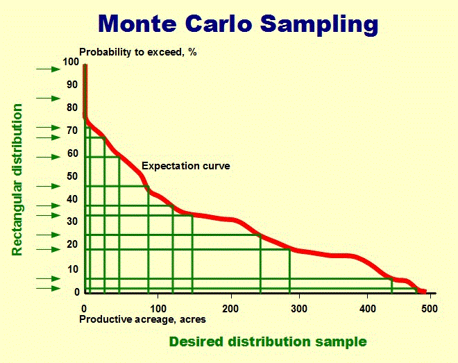
In mathematical terms, we need the inverse of the cdf. In that function the variable is the probability and we calculate that function for a value of the probability equal to the uniform random number. That is mathematically what we are doing graphically above.
While the MC method of random draws from an expectation curve as shown above will work for any kind of doistribution represented by a sorted vector of values, it may be possible to make draws from a distribution that is analytically defined.
Convenient distributions in MC simulation are the normal, the lognormal, triangular, double triangular and also the simple rectangular (uniform) distribution between 0 and 1. The latter is useful in simulating "yes/no" situations.
To start with the yes/no situation, a random 0 or 1 can be generated (rectangular distribution) to simulate a probability of success P (as a fraction). If the random number between 0 and 1 is less than P then the result is set to 1, otherwise to 0. You might consider the generated vector of 1 and 0 values as a "Yes/No" vector.
For the other distributions mentioned above we need the inverse cumulative distribution formula. This means that the random number represents a cumulative probability. This, inserted in the formula, generates the required random draw x from the distribution. For the details see the pages on the distributions mentioned above.
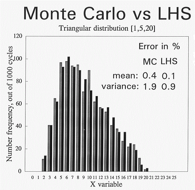
In the LHS case the resulting random draws are not coming in a random order, because the sampling interval are dealt with in sequence. For many follow-up calculations in the MC model it is required to "shake" the vector of random draws to get a random order by "sort and carry" routines.
If a calibration study found a useful relationship between a variable Y and a variable X then the regression equation can be used to predict in a MC simulation the value of Y given a value for X. The regression equation provide an estimate of the conditional mean of Y, given the X value. Then at this point a normal distribution is assumed with this mean and a standard deviation which is the standard error of estimate from the rgression, but with some adjustment. The formulas for this are explained under correlation.
The simple way to generate correlated vectors is based on sorting.
To correlate vectors X and Y with correlation coefficient r, sort r * n elements of each vector in ascending order, if n is the number of MC cycles. This assumes that both vectors were in independent random order before the sort. That the correlation r is equal to the percentage of the vector sorted follows from the formula for the correlation coefficient if the variables x and y are standardized:
The sorting does not affect the divisor. The only contribution to the denominator (covariance) is from the sorted part of the vector. The unsorted values for x and y are expected to be random and therefore will not contribute to the covariance. Hence r is equal to the percent sorted.
For many purposes this method is good enough. However, when a graph is drawn of the correlated vectors, i.e. Y versus X, a quite unnatural picture is obtained: the "Saturn effect". The correlated elements are forming an almost perfect straight line, while the unsorted parts form a almost circular cloud of points around it. It is looking at the planet Saturn from its side.
For a negative correlation, the sorted parts of the vectors have to be put into reverse order by a "flip routine".
The Saturn effect can be avoided by using a more sophisticated method as follows.Generating analytical distributions used in MC
Binomial Simulation
. Prediction based on a regression equation
Simulating a correlation between MC vectors

Assume we wish to simulate a correlation of r = 0.5 between two variables, X and Y, represented by vectors of random draws from their respective distributions. The algorithm is basically a combination of statistics and a sorting procedure:
a is the intercept and b the slope of the regression line of Y on X. Here we simulate what the Y vector would look like if it was correlated with required r with X.

