Input for trap capacity is in most cases a set of depths and areas of the top reservoir surface (contoured trap) in combination with a gross reservoir thickness. If also contours are given for the base reservoir, the stratigraphic trap option can be used, which is more or less a wedge-shaped reservoir. The following assumes a structural trap of which only the top reservoir shape is described. In similar folding style, the same information is describing the base reservoir, as this would be shifted down over the thickness of the gross reservoir, retaining its shape. In parallel folding this is not the case and the position of the base reservoir must be constructed to obtain depths/areas for the base reservoir.
Areas at top reservoir are given at a number of contour levels. The gross thickness g is a constant which has to be used to find the base reservoir. For similar folding this should be at a vertical distance g from the top reservoir, but for the parallel style it should be at a distance g perpendicular to the top reservoir, as explained in the Trap Description page:
Note that the parallel style, when a fold is narrow, can give rise to a "space deficiency" in the core of an anticline, which precludes a solution occasionally.
The following is a two-dimensional solution for the case of a contoured dip closure, where it is reasonable to assume an elliptic shape of the contour areas, or a half-ellipse for a fault closure. The case of a monocline is different and is treated separately.
Geometric construction of bottom reservoir surface
Calculating base reservoir from top reservoir
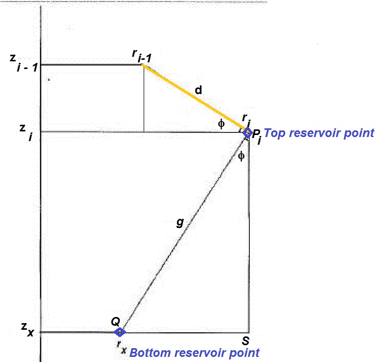
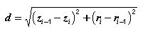
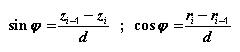
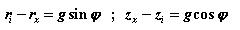
The coordinates we want to know are rx and zx, situated at the base of the reservoir. We note that the angle ( occurs in the triangle with the side d as well as in the triangle PiQS with the side g. From the two triangles we derive:
and the sine and cosine of φ.
Using the triangle PiQS we find:
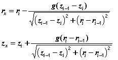
With these formulas the coordinates of the base points can be constructed for each point of the top reservoir. However a problem arises if the slope of the top reservoir changes, as it normally will do. In the first place, if the dip increases, there are too many zx at a given slice level and secondly, if the dip decreases, there are not enough zx to describe the base. If there is more than one base point for a given depth slice, we can choose to ignore the surplus, or, we might average them. In the case of too few, the gap may be closed by a simple linear, or more sophisticated interpolation. Some experimentation of a known model, such as the half sphere would indicate which solution is the most natural. A requirement might be, for instance, that dips of the base should not change too abruptly.
A boundary case can occur, given a steep dip of the top reservoir and a large g. Then rx can become negative. The depth zx will always be positive and hence does not present a problem. The meaning of a negative rx is the so-called "space deficiency" that can occur when layers are intensely folded. Here we can only set the rx to zero in such case. The consequence of this problem is that it becomes doubtful to apply the concentric folding to many reservoir/seal pairs. Geologically, a set of concentric folds stacked in a vertical sequence may not be tenable. However, a layered reservoir might be modeled as concentric.
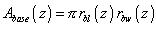
The area at a given depth is given for the top reservoir. For the bottom reservoir it has to be estimated by first obtaining the radius of the area as explained above. If the length and width of the trap are the same then the area becomes
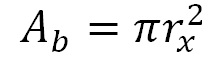
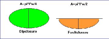
Most traps will have different shapes than circular domes. This means that the rx must be calculated for the length and for the width separately. Then we obtain the area as

where we use l for the length, w or the width of the trap and h for the vertical closure. The latter is about the same as the former. The dome is a good approximation, at least for the spherical segment or ellipsoid segment cases. We have to consider the difference between an all-round dip closure and a fault closure. The fault closure is modeled as half a dip closure with the cutting line in the length direction. Then the length is twice the half axis of the ellipse area and the width is the half axis perpendicular to the length, so, the meaning of w is different from that in the dip closure case:
Example of the half sphere.
When we use a trap model of half a sphere the following is found:
We take a sphere with radius 500 m. Then the "closure" is also 500 m. The depth at culmination is taken rather arbitrarily at 5000 m. The depth of the culmination has no effect on the calculations. What is important is the depth below the culmination at each contour. The areas at the contours are calculated at 11 intervals, starting with a zero area at the culmination and ending with the area of a circle with a radius of 500 m. To illustrate the effect of the different models we take a gross reservoir thickness of 100 m. If we would take 500 m, there would be no difference between the parallel and the similar models for the volume, the whole half sphere being filled with reservoir. We use the exact calculation of the contour radii to get the areas for each contour:
| Depth | Area |
| 5000 | 0.0000 |
| 5050 | 0.1492 |
| 5100 | 0.2827 |
| 5150 | 0.4005 |
| 5200 | 0.5026 |
| 5250 | 0.5890 |
| 5300 | 0.6597 |
| 5350 | 0.7147 |
| 5400 | 0.7540 |
| 5450 | 0.7775 |
| 5500 | 0.7854 |
The exact volume of the Bulk Reservoir Volume (BRV) should be 127.8.10^6 mł. The calculation using the contoured structural type give the following results:
| Similar model | 77.36 . 10^6 mł |
| Parallel model | 127.25 . 10^6 mł |
The parallel model is about half a percent too low. This is due to the interpolation and rounding errors. In structures with less extreme height to base ratio, i.e. less pronounced structures the error is likely to be much less. The important difference is, of course, between the similar and the parallel models: the 'similar' is only 60% of the 'parallel' model volume!
The Gaeapas user must therefore establish what kind of folding is expected, c.q. observed and accordingly use the model that fits best.
Three-dimensional solution.
Having the formulas for the 2-D solution, we must check whether this is sufficiently accurate for the case of a very narrow dip closure, i.e. where the length is several times as large as the width. For the top reservoir modeling, the areas are the input, and it does not matter what the shape of the area is. Areas in between the given input contours are interpolated. However, to determine the base reservoir configuration, the shape of the top reservoir is essential. If a spherical segment model is used to provide a radius for a given area at depth z, the radius will be different for the length and the width directions. Most important of all is that the radius of the sphere differs for the length and width directions. Now we may introduce the ratio s = w/l as the shape ratio. In this program the length and width are required, but not necessarily very accurately. After all,the areas of top reservoir area are given and we do not wish to override such values by any calculation (which would be the case if the length width, etc. are used in the simple spherical model as explained below). If the user does not provide the length and width, the program will assume a "dome" with length=width.
The 3-D solution now amounts to estimate the radius for the top reservoir area at depth z below culmination from the area A(z):
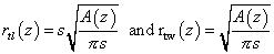
This is only an approximation that assumes that the ratio of width to length at any contour level is the same as at depth h below culmination. Note that for the spherical model, the ratio is a function of the depth z:
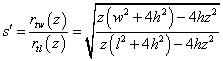
In the case of a contoured dip closure there is no justification for using the above to let the ratio vary with depth. So we use the approximation with constant ratio.
The modeling of the base is now done separately for the length and for the width directions. This gives the half axes for the elliptic areas of the base reservoir from which the areas are calculated: