Multiple Regression
The general form of multiple linear regression is:

The beta's are the coefficients in the regression equation with m variables. and are usually found by solving a matrix equation. The beta's derived from analysing a sample are only estimates. There is a standard deviation associated with each of the beta's. This gives useful information about the strength of the correlations between Y and the X's. A particularly useful measure is the "t-value" that is calculated by dividing the coefficient (beta) by it's standard deviation. It can be used as a test of significance and for estimating the amount of explained variance contributed by the X variable in question. The t-values, when squared, have a simple relationship with another statistic: the F-value. It would be beyond the scope of this note to go into further detail, but we draw attention to the importance of the t-values as indicators of the relative importance of X variables in a multivariate regression.
Most spreadsheets offer simple facilities to make a multiple regression, usually giving the following information:
| Regression Output | ||
|---|---|---|
| Constant | 0.295800 | |
| Std Error of Y Estimate | 1.107027 | |
| R Squared | 0.520452 | |
| No. of Observations | 12 | |
| Degrees of Freedom | 9 | |
| Independent variables | X1 | X2 |
| X Coefficient(s) | 0.404594 | 0.32088 |
| Std dev. of Coefficient | 0.200814 | 0.18468 |
| t-value | 2.014763 | 1.73746 |
The constant is in our notation beta0.
There were 12 sets of observations {Y,X1,X2} to work with. The number of Degrees of Freedom ("df") is 9. The df must be known of we wish to test for significant multiple correlation. We always loose one df for the mean of Y, and one for each X variable. In general, with n observations and m X-variables the df will be n-m-1. With this number of df, the t-tests on both X variables are significant at the 5% level, both variables contribute significantly to the explained variation of Y. If t-values are more than about 1.6, it is likely that the variable contributes to the prediction of Y.
The degree of freedom principle becomes a little clearer when we calculate a regression of Y on a single X variable with two observations. Then in sample space we have two points on a plane, representing the two observations. The regression line will be completely fixed by those two points: "perfect correlation", but meaningless as the df = n-m-1 = 2-1-1 = 0. When using multiple regression it is necessary to have a number of observations well exceeding the number of X-variables + 1, i.e. n >> m+1.
From such a table we can learn about the individual contributions of parameters to the explanation of Y (the partition of R-square) In the above example, 52% of the variation of Y is explained by X1 and X2. If we want the individual contributios we take the square of the t-values, sum these and then normalize as follows:
| Calculation of the contribution to uncertainty | |||
|---|---|---|---|
| Independent variable | t-value | t-value squared | Percent of R-square |
| X1 | 2.01476 | 4.05927 | 57.35% |
| X2 | 1.73746 | 3.01877 | 42.65% |
| Total | 7.07804 | 100% |
So, both together contribute about half the variance of Y, but X1 is somewhat stronger than X2. It could also occur that an X-variable has a very low t-value. Then it may be better not to use it in the regression. Some programs can automatically select the significant X variables.
Adjusted R-square
In the above example we have trusted R-square as giving us an unbiased indication of the variance in Y, explained by the two X's. This not exactly true. R-square can become "inflated" in the multivariate analysis. Hence it suggested to correct it to an adjusted R-square by using the following formula:
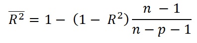
where adjusted R-square is indicated with a top bar, n the sample size and p the number of independent variables. The idea behind is that this correction is less biased than the "rough" R-square. As we are interested in the part of the variance of Y that is explained by the X's it is more direct to use the ratio of the variance of the residuals of the regression to the total variance of Y, giving the unexplained part and then taking the complement of that. The correction becomes more important with smaller samples and more independent variables. of Y.
The above example has only twelve observations and two explanatory variables. Applying the correction we get adjusted R-square = 0.413886 instead of 0.520452, or only 41% versus 52% explained variance!